Overview
SHAP (SHapley Additive exPlanations, see Lundberg and Lee (2017)) is an ingenious way to study black box models. SHAP values decompose - as fair as possible - predictions into additive feature contributions. Crunching SHAP values requires clever algorithms. Analyzing them, however, is super easy with the right visualizations. {shapviz} offers the latter.
In particular, the following plots are available:
-
sv_importance(): Importance plot (bar/beeswarm). -
sv_dependence()andsv_dependence2D(): Dependence plots to study feature effects and interactions. -
sv_interaction(): Interaction plot (beeswarm/bar). -
sv_waterfall(): Waterfall plot to study single or average predictions. -
sv_force(): Force plot as alternative to waterfall plot.
SHAP and feature values are stored in a “shapviz” object that is built from:
- Models that know how to calculate SHAP values: XGBoost, LightGBM, and h2o.
- SHAP crunchers like {fastshap}, {kernelshap}, {treeshap}, {fastr}, and {DALEX}.
- SHAP matrix and corresponding feature values.
We use {patchwork} to glue together multiple plots with (potentially) inconsistent x and/or color scale.
Installation
# From CRAN
install.packages("shapviz")

# Or the newest version from GitHub:
# install.packages("devtools")
devtools::install_github("ModelOriented/shapviz")
Usage
Shiny diamonds… let’s use XGBoost to model their prices by the four “C” variables.
Compact SHAP analysis
library(shapviz)
library(ggplot2)
library(xgboost)

set.seed(1)

xvars <- c("log_carat", "cut", "color", "clarity")
X <- diamonds |>
  transform(log_carat = log(carat)) |>
  subset(select = xvars)
head(X)
#>   log_carat       cut color clarity
#> 1 -1.469676     Ideal     E     SI2
#> 2 -1.560648   Premium     E     SI1
#> 3 -1.469676      Good     E     VS1
#> 4 -1.237874   Premium     I     VS2
#> 5 -1.171183      Good     J     SI2
#> 6 -1.427116 Very Good     J    VVS2

# Fit (untuned) model
fit <- xgb.train(
  params = list(learning_rate = 0.1, nthread = 1),
  data = xgb.DMatrix(data.matrix(X), label = log(diamonds$price), nthread = 1),
  nrounds = 65
)

# SHAP analysis: X can even contain factors
X_explain <- X[sample(nrow(X), 2000), ]
shp <- shapviz(fit, X_pred = data.matrix(X_explain), X = X_explain)

sv_importance(shp, show_numbers = TRUE)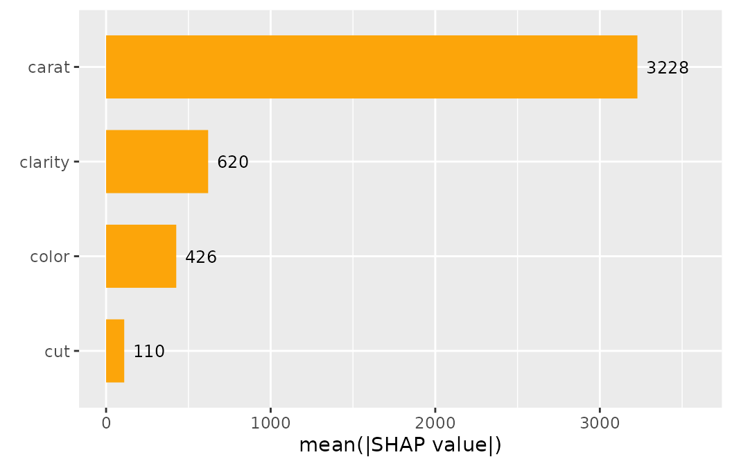
sv_importance(shp, kind = "beeswarm")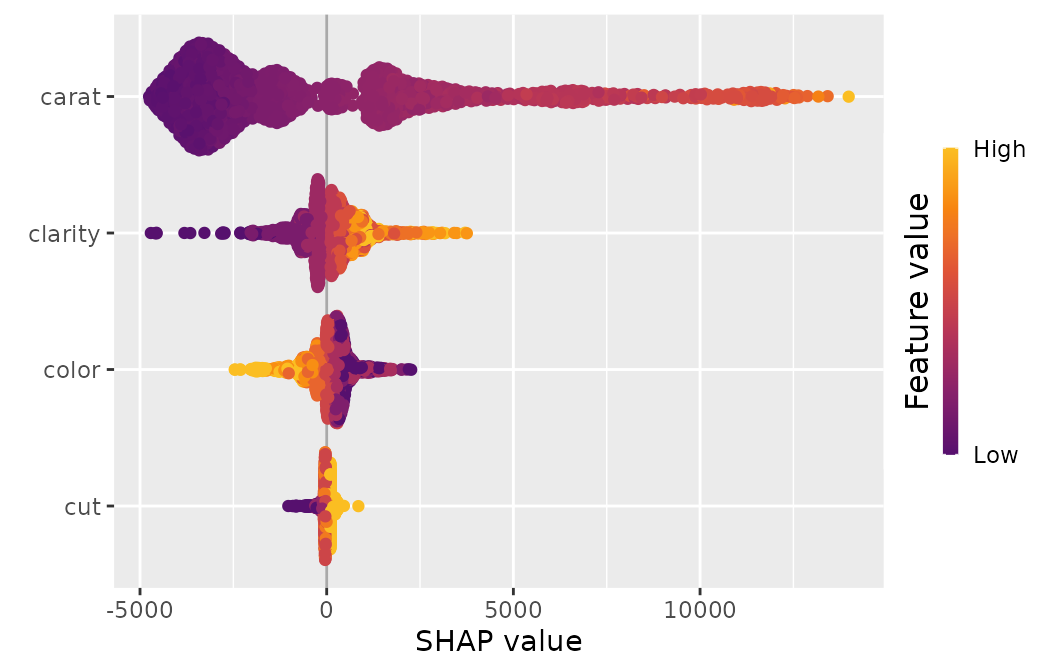
sv_dependence(shp, v = xvars, share_y = TRUE) # patchwork object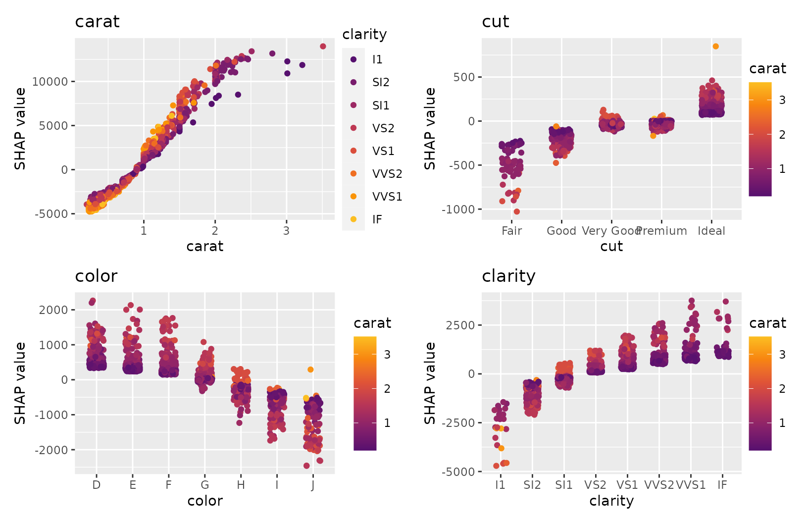
Decompose single predictions
We can visualize decompositions of single predictions via waterfall or force plots:
sv_waterfall(shp, row_id = 1) +
  theme(axis.text = element_text(size = 11))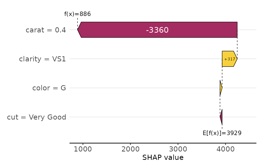
sv_force(shp, row_id = 1)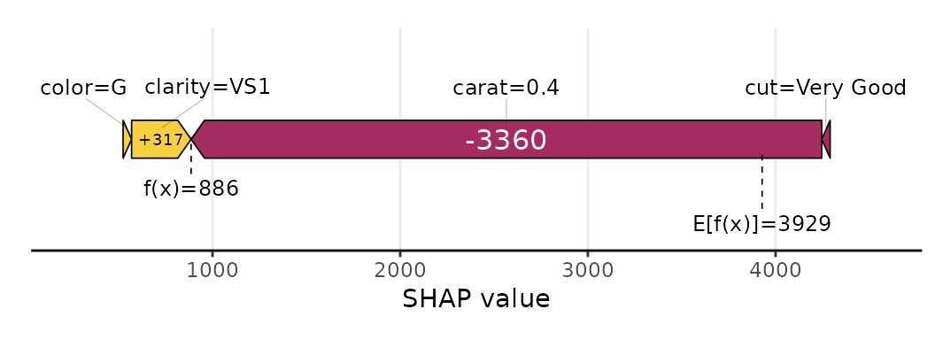
Also multiple row_id can be passed: The SHAP values of
the selected rows are averaged and then plotted as aggregated
SHAP values: The prediction profile for beautiful color “D”
diamonds:
sv_waterfall(shp, shp$X$color == "D") +
  theme(axis.text = element_text(size = 11))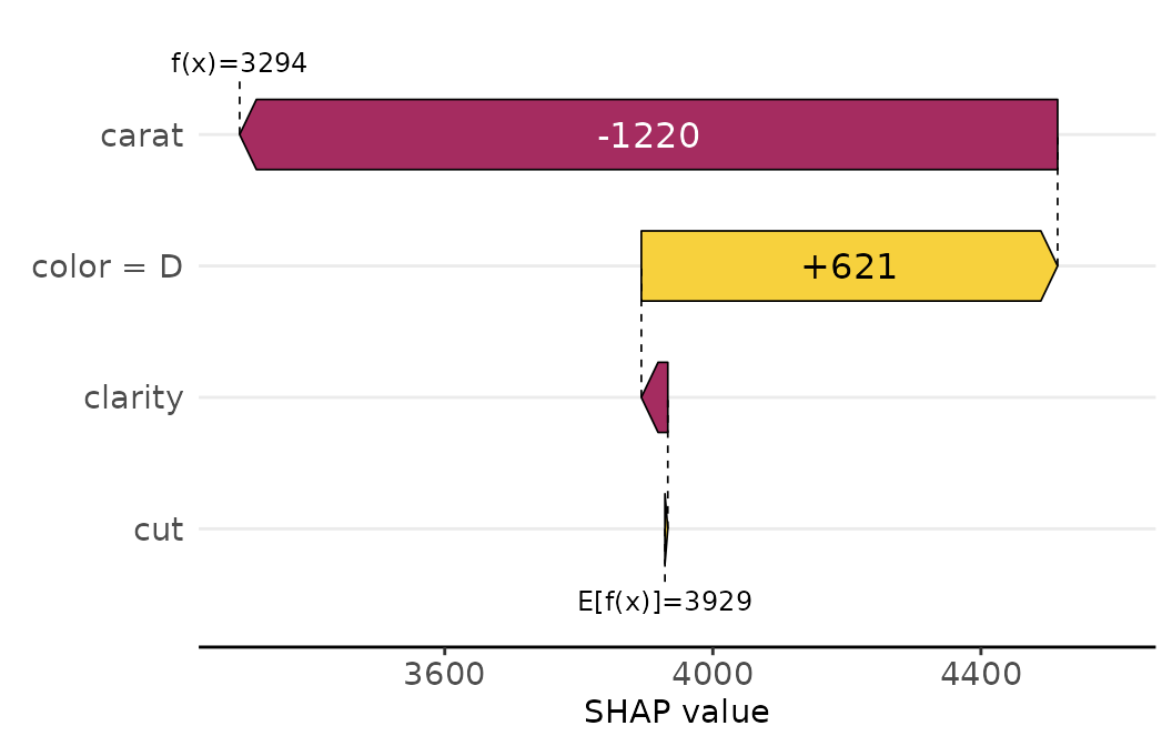
SHAP Interactions
If SHAP interaction values have been computed (via {xgboost} or
{treeshap}), we can study them by sv_dependence() and
sv_interaction().
Note that SHAP interaction values are multiplied by two (except main effects).
shp_i <- shapviz(
  fit, X_pred = data.matrix(X_explain), X = X_explain, interactions = TRUE
)
sv_dependence(shp_i, v = "log_carat", color_var = xvars, interactions = TRUE)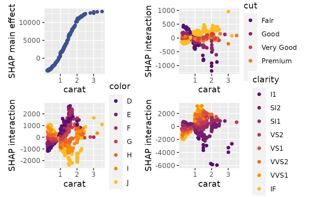
sv_interaction(shp_i)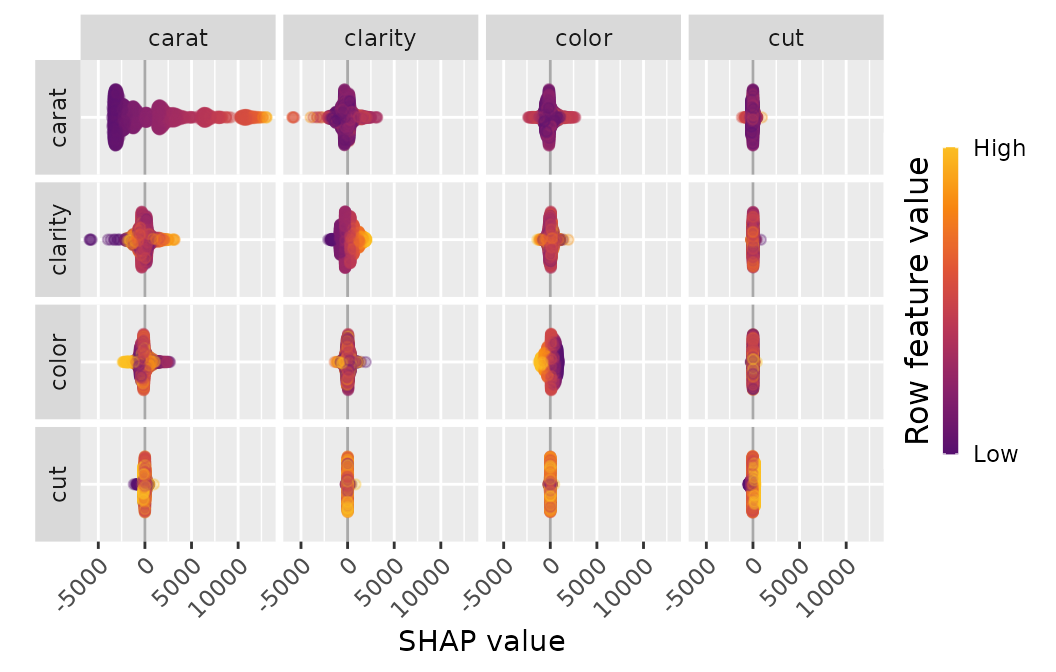
sv_interaction(shp_i, kind = "bar")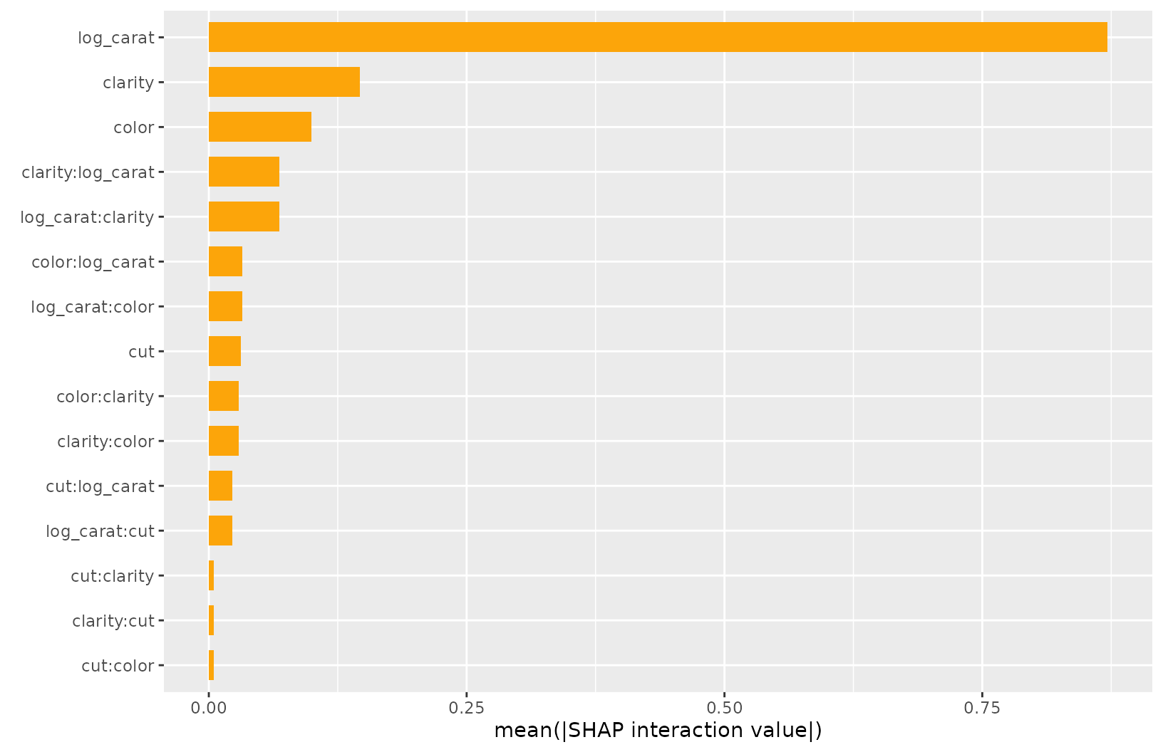
Interface to other packages
The above examples used XGBoost to calculate SHAP values. What about other packages?
LightGBM
library(shapviz)
library(lightgbm)

dtrain <- lgb.Dataset(data.matrix(iris[-1]), label = iris[, 1])
fit <- lgb.train(
  list(learning_rate = 0.1, objective = "mse"), data = dtrain, nrounds = 20
)
shp <- shapviz(fit, X_pred = data.matrix(iris[-1]), X = iris)
sv_importance(shp)shapr
library(shapviz)
library(shapr)

fit <- lm(Sepal.Length ~ ., data = iris)
explanation <- shapr::explain(
  model = fit,
  x_train = iris[-1],
  x_explain = iris[-1],
  approach = "ctree",
  phi0 = mean(iris$Sepal.Length)
)

shp <- shapviz(explanation)
sv_importance(shp)
sv_dependence(shp, "Sepal.Width")
H2O
H2O supports TreeSHAP for boosted trees and random forests. For other models, model agnostic method based on marginal expectations are used, requiring a background dataset.
library(shapviz)
library(h2o)

h2o.init()

iris2 <- as.h2o(iris)

# Random forest
xvars <- colnames(iris[-1])
fit_rf <- h2o.randomForest(xvars, "Sepal.Length", training_frame = iris2)
shp_rf <- shapviz(fit_rf, X_pred = iris)
sv_force(shp_rf, row_id = 1)
sv_dependence(shp_rf, xvars)

# Linear model
fit_lm <- h2o.glm(, "Sepal.Length", training_frame = iris2)
shp_lm <- shapviz(fit_lm, X_pred = iris, background_frame = iris2)
sv_force(shp_lm, row_id = 1)
sv_dependence(shp_lm, xvars)
treeshap
library(shapviz)
library(treeshap)
library(ranger)

fit <- ranger(
  y = iris$Sepal.Width, x = iris[-1], max.depth = 6, num.trees = 100
)
unified_model <- ranger.unify(fit, iris[-1])
shaps <- treeshap(unified_model, iris[-1], interactions = TRUE)
shp <- shapviz(shaps, X = iris)
sv_importance(shp)
sv_dependence(
  shp, "Sepal.Width", color_var = names(iris[-1]), alpha = 0.7, interactions = TRUE
)
DALEX
Decompositions of single predictions obtained by the breakdown algorithm in DALEX:
library(shapviz)
library(DALEX)
library(ranger)

fit <- ranger(Sepal.Length ~ ., data = iris, max.depth = 6, num.trees = 100)
explainer <- DALEX::explain(fit, data = iris[-1], y = iris[, 1], label = "RF")
bd <- explainer |>
  predict_parts(iris[1, ], keep_distributions = FALSE) |>
  shapviz()

sv_waterfall(bd)
sv_force(bd)
kernelshap
Either using kernelshap() or
permshap():
library(shapviz)
library(kernelshap)

set.seed(1)
fit <- lm(Sepal.Length ~ . + Species:Petal.Width, data = iris)
ks <- permshap(fit, iris[-1])
shp <- shapviz(ks)

sv_importance(shp)
sv_dependence(shp, colnames(iris[-1]))
Any other package
The most general interface is to provide a matrix of SHAP values and corresponding feature values (and optionally, a baseline value):
S <- matrix(c(1, -1, -1, 1), ncol = 2, dimnames = list(NULL, c("x", "y")))
X <- data.frame(x = c("a", "b"), y = c(100, 10))
shp <- shapviz(S, X, baseline = 4)
An example is CatBoost: it is not on CRAN, and requires
catboost.*() functions to calculate SHAP values, so we
cannot directly add it to {shapviz} for now. Use a wrapper like
this:
library(shapviz)
library(catboost)

shapviz.catboost.Model <- function(object, X_pred, X = X_pred, collapse = NULL, ...) {
  if (!inherits(X_pred, "catboost.Pool")) {
    X_pred <- catboost.load_pool(X_pred)
  }
  S <- catboost.get_feature_importance(object, X_pred, type = "ShapValues", ...)
  pp <- ncol(X_pred) + 1
  baseline <- S[1, pp]
  S <- S[, -pp, drop = FALSE]
  colnames(S) <- colnames(X_pred)
  shapviz(S, X = X, baseline = baseline, collapse = collapse)
}

# Example
X_pool <- catboost.load_pool(iris[-1], label = iris[, 1])
params <- list(loss_function = "RMSE", iterations = 65, allow_writing_files = FALSE)
fit <- catboost.train(X_pool, params = params)
shp <- shapviz(fit, X_pred = X_pool, X = iris)
sv_importance(shp)
sv_dependence(shp, colnames(iris[-1]))