This function creates an object of class "shapviz" from a matrix of SHAP values, or from a fitted model of type
XGBoost,
LightGBM, or
H2O.
Furthermore, shapviz() can digest the results of
shapr::explain(),treeshap::treeshap(),DALEX::predict_parts(),kernelshap::kernelshap(),kernelshap::permshap(), andkernelshap::additive_shap(),
check the vignettes for examples.
shapviz(object, ...)

# Default S3 method
shapviz(object, ...)

# S3 method for class 'matrix'
shapviz(object, X, baseline = 0, collapse = NULL, S_inter = NULL, ...)

# S3 method for class 'xgb.Booster'
shapviz(
  object,
  X_pred,
  X = X_pred,
  which_class = NULL,
  collapse = NULL,
  interactions = FALSE,
  ...
)

# S3 method for class 'lgb.Booster'
shapviz(object, X_pred, X = X_pred, which_class = NULL, collapse = NULL, ...)

# S3 method for class 'explain'
shapviz(object, X = NULL, baseline = NULL, collapse = NULL, ...)

# S3 method for class 'treeshap'
shapviz(
  object,
  X = object[["observations"]],
  baseline = 0,
  collapse = NULL,
  ...
)

# S3 method for class 'predict_parts'
shapviz(object, ...)

# S3 method for class 'shapr'
shapviz(
  object,
  X = as.data.frame(object$internal$data$x_explain),
  collapse = NULL,
  ...
)

# S3 method for class 'kernelshap'
shapviz(object, X = object[["X"]], which_class = NULL, collapse = NULL, ...)

# S3 method for class 'H2OModel'
shapviz(
  object,
  X_pred,
  X = as.data.frame(X_pred),
  collapse = NULL,
  background_frame = NULL,
  output_space = FALSE,
  output_per_reference = FALSE,
  ...
)
Arguments
- object
For XGBoost, LightGBM, and H2O, this is the fitted model used to calculate SHAP values from
X_pred. In the other cases, it is the object containing the SHAP values.- ...
Parameters passed to other methods (currently only used by the
predict()functions of XGBoost, LightGBM, and H2O).- X
Matrix or data.frame of feature values used for visualization. Must contain at least the same column names as the SHAP matrix represented by
object/X_pred(after optionally collapsing some of the SHAP columns).- baseline
Optional baseline value, representing the average response at the scale of the SHAP values. It will be used for plot methods that explain single predictions.
- collapse
A named list of character vectors. Each vector specifies the feature names whose SHAP values need to be summed up. The names determine the resulting collapsed column/dimension names.
- S_inter
Optional 3D array of SHAP interaction values. If
objecthas shape n x p, thenS_interneeds to be of shape n x p x p. Summation over the second (or third) dimension should yield the usual SHAP values. Furthermore, dimensions 2 and 3 are expected to be symmetric. Default isNULL.- X_pred
Data set as expected by the
predict()function of XGBoost, LightGBM, or H2O. For XGBoost, a matrix orxgb.DMatrix, for LightGBM a matrix, and for H2O adata.frameor anH2OFrame. Only used for XGBoost, LightGBM, or H2O objects.- which_class
In case of a multiclass or multioutput setting, which class/output (>= 1) to explain. Currently relevant for XGBoost, LightGBM, kernelshap, and permshap.
- interactions
Should SHAP interactions be calculated (default is
FALSE)? Only available for XGBoost.- background_frame
Background dataset for baseline SHAP or marginal SHAP. Only for H2O models.
- output_space
If model has link function, this argument controls whether the SHAP values should be linearly (= approximately) transformed to the original scale (if
TRUE). The default is to return the values on link scale. Only for H2O models.- output_per_reference
Switches between different algorithms, see
?h2o::h2o.predict_contributionsfor details. Only for H2O models.
Value
An object of class "shapviz" with the following elements:
S: Numeric matrix of SHAP values.X:data.framecontaining the feature values corresponding toS.baseline: Baseline value, representing the average prediction at the scale of the SHAP values.S_inter: Numeric array of SHAP interaction values (orNULL).
Details
Together with the main input, a data set X of feature values is required,
used only for visualization. It can therefore contain character or factor
variables, even if the SHAP values were calculated from a purely numerical feature
matrix. In addition, to improve visualization, it can sometimes be useful to truncate
gross outliers, logarithmize certain columns, or replace missing values with an
explicit value.
SHAP values of dummy variables can be combined using the convenient
collapse argument.
Multi-output models created from XGBoost, LightGBM, "kernelshap", or "permshap"
return a "mshapviz" object, containing a "shapviz" object per output.
Methods (by class)
shapviz(default): Default method to initialize a "shapviz" object.shapviz(matrix): Creates a "shapviz" object from a matrix of SHAP values.shapviz(xgb.Booster): Creates a "shapviz" object from an XGBoost model.shapviz(lgb.Booster): Creates a "shapviz" object from a LightGBM model.shapviz(explain): Creates a "shapviz" object fromfastshap::explain().shapviz(treeshap): Creates a "shapviz" object fromtreeshap::treeshap().shapviz(predict_parts): Creates a "shapviz" object fromDALEX::predict_parts().shapviz(shapr): Creates a "shapviz" object fromshapr::explain().shapviz(kernelshap): Creates a "shapviz" object from an object of class 'kernelshap'. This includes results ofkernelshap(),permshap(), andadditive_shap().shapviz(H2OModel): Creates a "shapviz" object from an H2O model.
See also
Examples
S <- matrix(c(1, -1, -1, 1), ncol = 2, dimnames = list(NULL, c("x", "y")))
X <- data.frame(x = c("a", "b"), y = c(100, 10))
shapviz(S, X, baseline = 4)
#> 'shapviz' object representing 2 x 2 SHAP matrix. Top lines:
#>
#> x y
#> [1,] 1 -1
#> [2,] -1 1
# XGBoost models
X_pred <- data.matrix(iris[, -1])
dtrain <- xgboost::xgb.DMatrix(X_pred, label = iris[, 1], nthread = 1)
fit <- xgboost::xgb.train(list(nthread = 1), data = dtrain, nrounds = 10)
# Will use numeric matrix "X_pred" as feature matrix
x <- shapviz(fit, X_pred = X_pred)
x
#> 'shapviz' object representing 150 x 4 SHAP matrix. Top lines:
#>
#> Sepal.Width Petal.Length Petal.Width Species
#> [1,] 0.05504481 -0.7191185 -0.0629074 0.004168344
#> [2,] -0.13272415 -0.7881535 -0.1101536 0.006157321
sv_dependence(x, "Species")
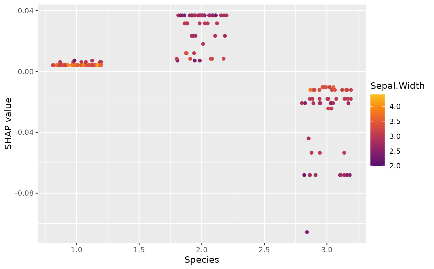 # Will use original values as feature matrix
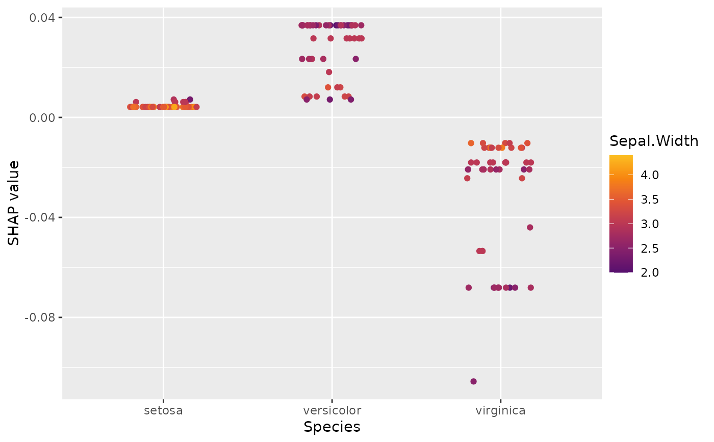
x <- shapviz(fit, X_pred = X_pred, X = iris)
sv_dependence(x, "Species")
# Will use original values as feature matrix
x <- shapviz(fit, X_pred = X_pred, X = iris)
sv_dependence(x, "Species")
 # "X_pred" can also be passed as xgb.DMatrix, but only if X is passed as well!
x <- shapviz(fit, X_pred = dtrain, X = iris)
# Multiclass setting
params <- list(objective = "multi:softprob", num_class = 3, nthread = 1)
X_pred <- data.matrix(iris[, -5])
dtrain <- xgboost::xgb.DMatrix(
X_pred, label = as.integer(iris[, 5]) - 1, nthread = 1
)
fit <- xgboost::xgb.train(params = params, data = dtrain, nrounds = 10)
# Select specific class
x <- shapviz(fit, X_pred = X_pred, which_class = 3)
x
#> 'shapviz' object representing 150 x 4 SHAP matrix. Top lines:
#>
#> Sepal.Length Sepal.Width Petal.Length Petal.Width
#> [1,] -0.02178742 0 -1.14285 -0.4735336
#> [2,] -0.02178742 0 -1.14285 -0.4735336
# Or combine all classes to "mshapviz" object
x <- shapviz(fit, X_pred = X_pred)
x
#> 'mshapviz' object representing 3 'shapviz' objects:
#> 'Class_1': 150 x 4 SHAP matrix
#> 'Class_2': 150 x 4 SHAP matrix
#> 'Class_3': 150 x 4 SHAP matrix
# What if we would have one-hot-encoded values and want to explain the original column?
X_pred <- stats::model.matrix(~ . -1, iris[, -1])
dtrain <- xgboost::xgb.DMatrix(X_pred, label = as.integer(iris[, 1]), nthread = 1)
fit <- xgboost::xgb.train(list(nthread = 1), data = dtrain, nrounds = 10)
x <- shapviz(
fit,
X_pred = X_pred,
X = iris,
collapse = list(Species = c("Speciessetosa", "Speciesversicolor", "Speciesvirginica"))
)
summary(x)
#> 'shapviz' object representing
#> - SHAP matrix of dimension 150 x 4
#> - feature data.frame of dimension 150 x 4
#> - baseline value of 5.219078
#>
#> SHAP values of first 2 observations:
#> Sepal.Width Petal.Length Petal.Width Species
#> [1,] 0.2483077 -0.5881364 -0.06978062 -0.02456470
#> [2,] -0.2360498 -0.7144780 -0.20988548 -0.05386889
#>
#> Corresponding feature values:
#> Sepal.Width Petal.Length Petal.Width Species
#> 1 3.5 1.4 0.2 setosa
#> 2 3.0 1.4 0.2 setosa
#>
# Similarly with LightGBM
if (requireNamespace("lightgbm", quietly = TRUE)) {
fit <- lightgbm::lgb.train(
params = list(objective = "regression", num_thread = 1),
data = lightgbm::lgb.Dataset(X_pred, label = iris[, 1]),
nrounds = 10,
verbose = -2
)
x <- shapviz(fit, X_pred = X_pred)
x
# Multiclass
params <- list(objective = "multiclass", num_class = 3, num_thread = 1)
X_pred <- data.matrix(iris[, -5])
dtrain <- lightgbm::lgb.Dataset(X_pred, label = as.integer(iris[, 5]) - 1)
fit <- lightgbm::lgb.train(params = params, data = dtrain, nrounds = 10)
# Select specific class
x <- shapviz(fit, X_pred = X_pred, which_class = 3)
x
# Or combine all classes to a "mshapviz" object
mx <- shapviz(fit, X_pred = X_pred)
mx
all.equal(mx[[3]], x)
}
#> [LightGBM] [Info] Auto-choosing col-wise multi-threading, the overhead of testing was 0.000020 seconds.
#> You can set `force_col_wise=true` to remove the overhead.
#> [LightGBM] [Info] Total Bins 98
#> [LightGBM] [Info] Number of data points in the train set: 150, number of used features: 4
#> [LightGBM] [Info] Start training from score -1.098612
#> [LightGBM] [Info] Start training from score -1.098612
#> [LightGBM] [Info] Start training from score -1.098612
#> [LightGBM] [Warning] No further splits with positive gain, best gain: -inf
#> [LightGBM] [Warning] No further splits with positive gain, best gain: -inf
#> [LightGBM] [Warning] No further splits with positive gain, best gain: -inf
#> [LightGBM] [Warning] No further splits with positive gain, best gain: -inf
#> [LightGBM] [Warning] No further splits with positive gain, best gain: -inf
#> [LightGBM] [Warning] No further splits with positive gain, best gain: -inf
#> [LightGBM] [Warning] No further splits with positive gain, best gain: -inf
#> [LightGBM] [Warning] No further splits with positive gain, best gain: -inf
#> [LightGBM] [Warning] No further splits with positive gain, best gain: -inf
#> [LightGBM] [Warning] No further splits with positive gain, best gain: -inf
#> [LightGBM] [Warning] No further splits with positive gain, best gain: -inf
#> [LightGBM] [Warning] No further splits with positive gain, best gain: -inf
#> [LightGBM] [Warning] No further splits with positive gain, best gain: -inf
#> [LightGBM] [Warning] No further splits with positive gain, best gain: -inf
#> [LightGBM] [Warning] No further splits with positive gain, best gain: -inf
#> [LightGBM] [Warning] No further splits with positive gain, best gain: -inf
#> [LightGBM] [Warning] No further splits with positive gain, best gain: -inf
#> [LightGBM] [Warning] No further splits with positive gain, best gain: -inf
#> [LightGBM] [Warning] No further splits with positive gain, best gain: -inf
#> [LightGBM] [Warning] No further splits with positive gain, best gain: -inf
#> [LightGBM] [Warning] No further splits with positive gain, best gain: -inf
#> [LightGBM] [Warning] No further splits with positive gain, best gain: -inf
#> [LightGBM] [Warning] No further splits with positive gain, best gain: -inf
#> [LightGBM] [Warning] No further splits with positive gain, best gain: -inf
#> [LightGBM] [Warning] No further splits with positive gain, best gain: -inf
#> [LightGBM] [Warning] No further splits with positive gain, best gain: -inf
#> [LightGBM] [Warning] No further splits with positive gain, best gain: -inf
#> [LightGBM] [Warning] No further splits with positive gain, best gain: -inf
#> [LightGBM] [Warning] No further splits with positive gain, best gain: -inf
#> [LightGBM] [Warning] No further splits with positive gain, best gain: -inf
#> [1] TRUE
# "X_pred" can also be passed as xgb.DMatrix, but only if X is passed as well!
x <- shapviz(fit, X_pred = dtrain, X = iris)
# Multiclass setting
params <- list(objective = "multi:softprob", num_class = 3, nthread = 1)
X_pred <- data.matrix(iris[, -5])
dtrain <- xgboost::xgb.DMatrix(
X_pred, label = as.integer(iris[, 5]) - 1, nthread = 1
)
fit <- xgboost::xgb.train(params = params, data = dtrain, nrounds = 10)
# Select specific class
x <- shapviz(fit, X_pred = X_pred, which_class = 3)
x
#> 'shapviz' object representing 150 x 4 SHAP matrix. Top lines:
#>
#> Sepal.Length Sepal.Width Petal.Length Petal.Width
#> [1,] -0.02178742 0 -1.14285 -0.4735336
#> [2,] -0.02178742 0 -1.14285 -0.4735336
# Or combine all classes to "mshapviz" object
x <- shapviz(fit, X_pred = X_pred)
x
#> 'mshapviz' object representing 3 'shapviz' objects:
#> 'Class_1': 150 x 4 SHAP matrix
#> 'Class_2': 150 x 4 SHAP matrix
#> 'Class_3': 150 x 4 SHAP matrix
# What if we would have one-hot-encoded values and want to explain the original column?
X_pred <- stats::model.matrix(~ . -1, iris[, -1])
dtrain <- xgboost::xgb.DMatrix(X_pred, label = as.integer(iris[, 1]), nthread = 1)
fit <- xgboost::xgb.train(list(nthread = 1), data = dtrain, nrounds = 10)
x <- shapviz(
fit,
X_pred = X_pred,
X = iris,
collapse = list(Species = c("Speciessetosa", "Speciesversicolor", "Speciesvirginica"))
)
summary(x)
#> 'shapviz' object representing
#> - SHAP matrix of dimension 150 x 4
#> - feature data.frame of dimension 150 x 4
#> - baseline value of 5.219078
#>
#> SHAP values of first 2 observations:
#> Sepal.Width Petal.Length Petal.Width Species
#> [1,] 0.2483077 -0.5881364 -0.06978062 -0.02456470
#> [2,] -0.2360498 -0.7144780 -0.20988548 -0.05386889
#>
#> Corresponding feature values:
#> Sepal.Width Petal.Length Petal.Width Species
#> 1 3.5 1.4 0.2 setosa
#> 2 3.0 1.4 0.2 setosa
#>
# Similarly with LightGBM
if (requireNamespace("lightgbm", quietly = TRUE)) {
fit <- lightgbm::lgb.train(
params = list(objective = "regression", num_thread = 1),
data = lightgbm::lgb.Dataset(X_pred, label = iris[, 1]),
nrounds = 10,
verbose = -2
)
x <- shapviz(fit, X_pred = X_pred)
x
# Multiclass
params <- list(objective = "multiclass", num_class = 3, num_thread = 1)
X_pred <- data.matrix(iris[, -5])
dtrain <- lightgbm::lgb.Dataset(X_pred, label = as.integer(iris[, 5]) - 1)
fit <- lightgbm::lgb.train(params = params, data = dtrain, nrounds = 10)
# Select specific class
x <- shapviz(fit, X_pred = X_pred, which_class = 3)
x
# Or combine all classes to a "mshapviz" object
mx <- shapviz(fit, X_pred = X_pred)
mx
all.equal(mx[[3]], x)
}
#> [LightGBM] [Info] Auto-choosing col-wise multi-threading, the overhead of testing was 0.000020 seconds.
#> You can set `force_col_wise=true` to remove the overhead.
#> [LightGBM] [Info] Total Bins 98
#> [LightGBM] [Info] Number of data points in the train set: 150, number of used features: 4
#> [LightGBM] [Info] Start training from score -1.098612
#> [LightGBM] [Info] Start training from score -1.098612
#> [LightGBM] [Info] Start training from score -1.098612
#> [LightGBM] [Warning] No further splits with positive gain, best gain: -inf
#> [LightGBM] [Warning] No further splits with positive gain, best gain: -inf
#> [LightGBM] [Warning] No further splits with positive gain, best gain: -inf
#> [LightGBM] [Warning] No further splits with positive gain, best gain: -inf
#> [LightGBM] [Warning] No further splits with positive gain, best gain: -inf
#> [LightGBM] [Warning] No further splits with positive gain, best gain: -inf
#> [LightGBM] [Warning] No further splits with positive gain, best gain: -inf
#> [LightGBM] [Warning] No further splits with positive gain, best gain: -inf
#> [LightGBM] [Warning] No further splits with positive gain, best gain: -inf
#> [LightGBM] [Warning] No further splits with positive gain, best gain: -inf
#> [LightGBM] [Warning] No further splits with positive gain, best gain: -inf
#> [LightGBM] [Warning] No further splits with positive gain, best gain: -inf
#> [LightGBM] [Warning] No further splits with positive gain, best gain: -inf
#> [LightGBM] [Warning] No further splits with positive gain, best gain: -inf
#> [LightGBM] [Warning] No further splits with positive gain, best gain: -inf
#> [LightGBM] [Warning] No further splits with positive gain, best gain: -inf
#> [LightGBM] [Warning] No further splits with positive gain, best gain: -inf
#> [LightGBM] [Warning] No further splits with positive gain, best gain: -inf
#> [LightGBM] [Warning] No further splits with positive gain, best gain: -inf
#> [LightGBM] [Warning] No further splits with positive gain, best gain: -inf
#> [LightGBM] [Warning] No further splits with positive gain, best gain: -inf
#> [LightGBM] [Warning] No further splits with positive gain, best gain: -inf
#> [LightGBM] [Warning] No further splits with positive gain, best gain: -inf
#> [LightGBM] [Warning] No further splits with positive gain, best gain: -inf
#> [LightGBM] [Warning] No further splits with positive gain, best gain: -inf
#> [LightGBM] [Warning] No further splits with positive gain, best gain: -inf
#> [LightGBM] [Warning] No further splits with positive gain, best gain: -inf
#> [LightGBM] [Warning] No further splits with positive gain, best gain: -inf
#> [LightGBM] [Warning] No further splits with positive gain, best gain: -inf
#> [LightGBM] [Warning] No further splits with positive gain, best gain: -inf
#> [1] TRUE