Multiple ‘shapviz’ objects

Overview

Sometimes, you will find it necessary to work with several “shapviz” objects at the same time:

• To visualize SHAP values of a multiclass or multi-output model.
• To compare SHAP plots of different models with common features.
• To study SHAP plots between subgroups.

To simplify the workflow, {shapviz} offers a “mshapviz” object (“m” like “multi”). You can create it in different ways:

• Use shapviz() on multiclass XGBoost or LightGBM models.
• Use shapviz() on “kernelshap” or “permshap” objects created from multiclass/multioutput models via the {kernelshap} package.
• Use c(Mod_1 = s1, Mod_2 = s2, ...) on “shapviz” objects s1, s2, …
• Or mshapviz(list(Mod_1 = s1, Mod_2 = s2, ...))

The sv_*() functions mainly use the {patchwork} package to glue the individual plots together. An exception is sv_importance(..., kind = "bar"), which produces a dodged barplot via {ggplot2}, by default.

Example: Multiclass XGBoost model

library(shapviz)
library(ggplot2)
library(patchwork)
library(xgboost)

params <- list(objective = "multi:softprob", num_class = 3, nthread = 1)
X_pred <- data.matrix(iris[, -5])
dtrain <- xgb.DMatrix(X_pred, label = as.integer(iris[, 5]) - 1, nthread = 1)
fit <- xgb.train(params = params, data = dtrain, nrounds = 50)

# Create "mshapviz" object (logit scale)
(x <- shapviz(fit, X_pred = X_pred, X = iris))
#> 'mshapviz' object representing 3 'shapviz' objects:
#>    'Class_1': 150 x 4 SHAP matrix
#>    'Class_2': 150 x 4 SHAP matrix
#>    'Class_3': 150 x 4 SHAP matrix

# Contains "shapviz" objects for all classes
all.equal(x[[3]], shapviz(fit, X_pred = X_pred, X = iris, which_class = 3))
#> [1] TRUE

# Better names
names(x) <- levels(iris$Species)
x
#> 'mshapviz' object representing 3 'shapviz' objects:
#>    'setosa': 150 x 4 SHAP matrix
#>    'versicolor': 150 x 4 SHAP matrix
#>    'virginica': 150 x 4 SHAP matrix

# SHAP plots
sv_importance(x)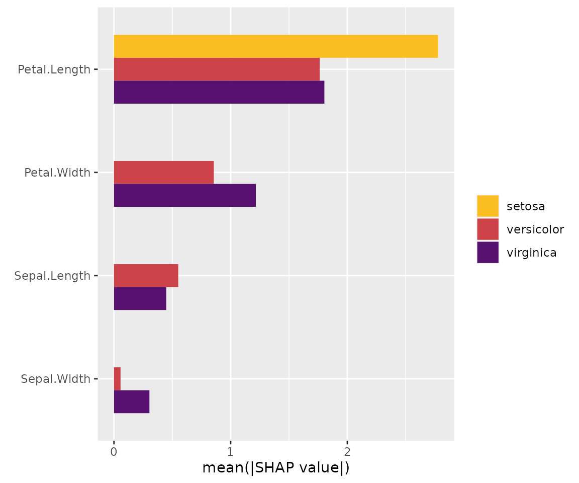

sv_importance(x, bar_type = "stack")  # Same but stacked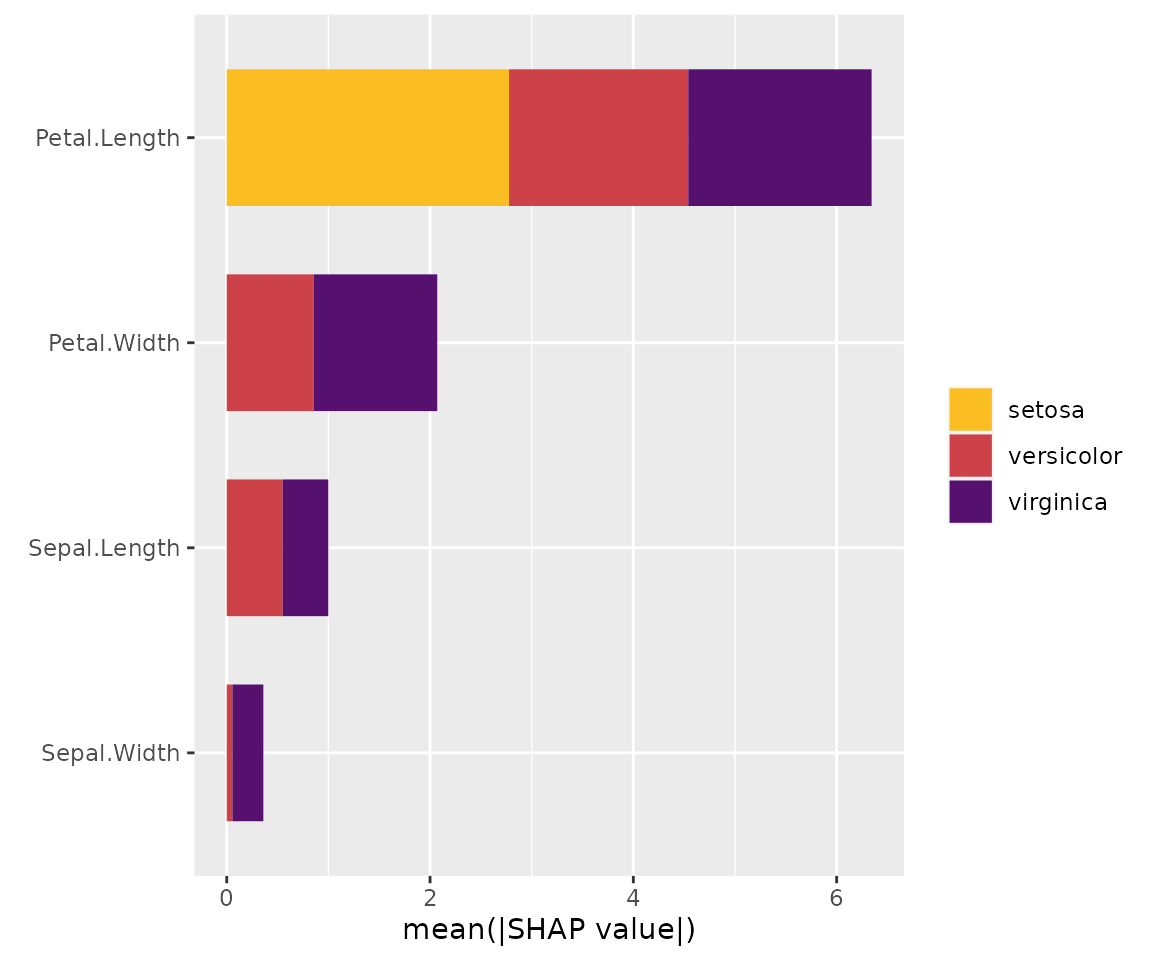

sv_dependence(x, v = "Petal.Length") +
  plot_layout(ncol = 1) &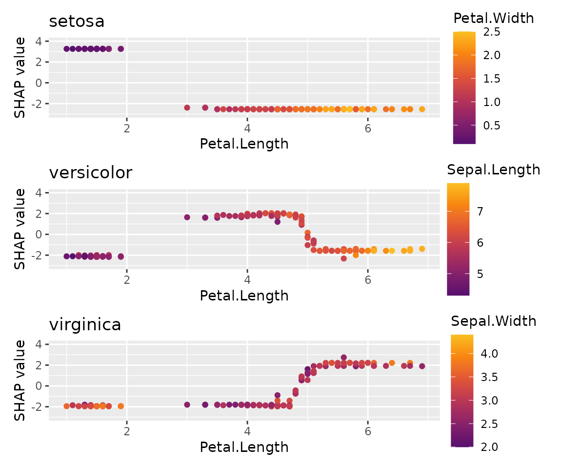
  ylim(-3, 4)  # Same y scale to get impression on strength

Similar for LightGBM (only code)

library(shapviz)
library(lightgbm)

# Model
params <- list(objective = "multiclass", num_class = 3)
X_pred <- data.matrix(iris[, -5])
dtrain <- lgb.Dataset(X_pred, label = as.integer(iris[, 5]) - 1)
fit <- lgb.train(params = params, data = dtrain, nrounds = 50)

x <- shapviz(fit, X_pred = X_pred, X = iris)

sv_importance(x)

Or for a random forest with {kernelshap}

Since Kernel SHAP is model agnostic, we get SHAP values on probability scale. To explain log-odds, we would need to pass our own predict function to kernelshap().

library(shapviz)
library(kernelshap)
library(ggplot2)
library(patchwork)
library(ranger)

# Model
fit <- ranger(Species ~ ., data = iris, num.trees = 100, probability = TRUE, seed = 1)

# "mshapviz" object
x <- kernelshap(fit, X = iris[-5], bg_X = iris)
shp <- setNames(shapviz(x), levels(iris$Species))
# all.equal(shp[[3]], shapviz(x, which_class = 3))

sv_importance(shp)

sv_dependence(shp, v = "Sepal.Width") +
  plot_layout(ncol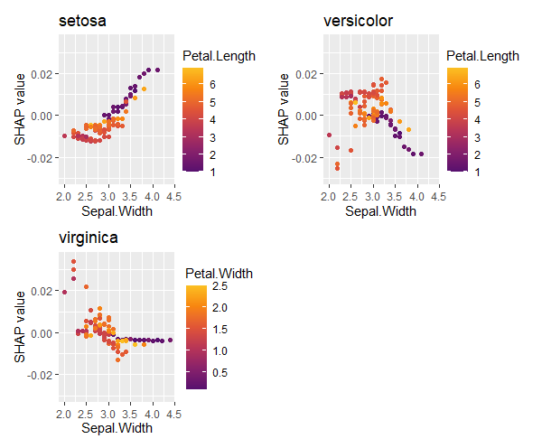 = 2) &
  ylim(-0.06, 0.06)

Example: SHAP subgroup analysis

Let’s compare SHAP dependence plots across Species.

library(shapviz)
library(ggplot2)
library(patchwork)
library(xgboost)

X_pred <- data.matrix(iris[, -1])
dtrain <- xgb.DMatrix(X_pred, label = iris[, 1], nthread = 1)
fit_xgb <- xgb.train(params = list(nthread = 1), data = dtrain, nrounds = 50)

# Create "mshapviz" object and split it into subgroups
shap_xgb <- shapviz(fit_xgb, X_pred = X_pred, X = iris)
x_subgroups <- split(shap_xgb, f = iris$Species)

# SHAP analysis
sv_importance(x_subgroups, bar_type = "stack")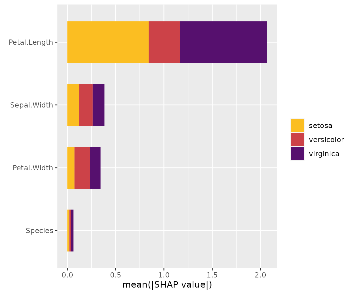

sv_dependence(x_subgroups, v = "Petal.Length") +
  plot_layout(ncol = 1) & 
  xlim(1, 7) &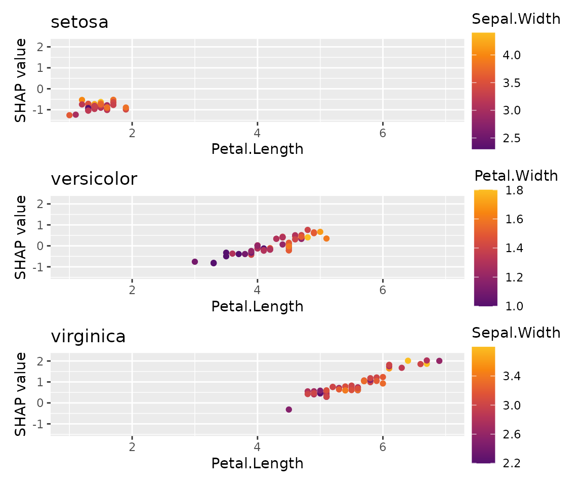
  ylim(-1.4, 2.2)

Example: Different models

In the last example, we used a regression model fitted via XGBoost. How does it compare with a linear regression?

Fit linear regression and use {kernelshap} to get SHAP values

library(kernelshap)

fit_lm <- lm(Sepal.Length ~ ., data = iris)
shap_lm <- shapviz(kernelshap(fit_lm, iris[-1], bg_X = iris))

# Combine "shapviz" objects
mshap <- c(lm = shap_lm, xgb = shap_xgb)
mshap

#> 'mshapviz' object representing 2 'shapviz' objects:
#>   'lm': 150 x 4 SHAP matrix
#>   'xgb': 150 x 4 SHAP matrix

# SHAP analysis
sv_importance(mshap)

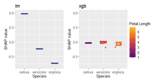
sv_dependence(mshap, v = "Species") &
  ylim(-0.5, 0.6)