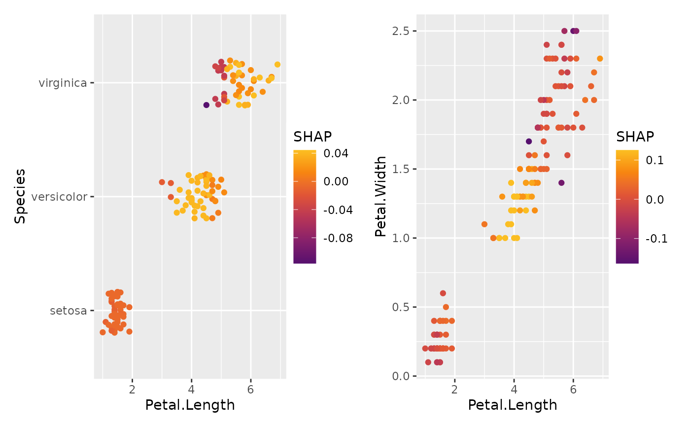
Scatterplot of two features, showing the sum of their SHAP values on the color scale.
This allows to visualize the combined effect of two features, including interactions.
A typical application are models with latitude and longitude as features (plus
maybe other regional features that can be passed via add_vars).
If SHAP interaction values are available, setting interactions = TRUE allows
to focus on pure interaction effects (multiplied by two). In this case, add_vars
has no effect.
sv_dependence2D(object, ...)

# Default S3 method
sv_dependence2D(object, ...)

# S3 method for class 'shapviz'
sv_dependence2D(
  object,
  x,
  y,
  viridis_args = getOption("shapviz.viridis_args"),
  jitter_width = NULL,
  jitter_height = NULL,
  interactions = FALSE,
  add_vars = NULL,
  seed = 1L,
  ...
)

# S3 method for class 'mshapviz'
sv_dependence2D(
  object,
  x,
  y,
  viridis_args = getOption("shapviz.viridis_args"),
  jitter_width = NULL,
  jitter_height = NULL,
  interactions = FALSE,
  add_vars = NULL,
  seed = 1L,
  ...
)
Arguments
- object
An object of class "(m)shapviz".
- ...
Arguments passed to
ggplot2::geom_jitter().- x
Feature name for x axis. Can be a vector if
objectis of class "shapviz".- y
Feature name for y axis. Can be a vector if
objectis of class "shapviz".- viridis_args
List of viridis color scale arguments, see
?ggplot2::scale_color_viridis_c. The default points to the global optionshapviz.viridis_args, which corresponds tolist(begin = 0.25, end = 0.85, option = "inferno"). These values are passed toggplot2::scale_color_viridis_*(). For example, to switch to a standard viridis scale, you can either change the default viaoptions(shapviz.viridis_args = list()), or setviridis_args = list(). Only relevant ifcolor_varis notNULL.- jitter_width
The amount of horizontal jitter. The default (
NULL) will use a value of 0.2 in casevis discrete, and no jitter otherwise. (Numeric variables are considered discrete if they have at most 7 unique values.) Can be a vector/list ifvis a vector.- jitter_height
Similar to
jitter_widthfor vertical scatter.- interactions
Should SHAP interaction values be plotted? The default (
FALSE) will show the rowwise sum of the SHAP values ofxandy. IfTRUE, will use twice the SHAP interaction value (requires SHAP interactions).- add_vars
Optional vector of feature names, whose SHAP values should be added to the sum of the SHAP values of
xandy(only ifinteractions = FALSE). A use case would be a model with geographic x and y coordinates, along with some additional locational features like distance to the next train station.- seed
Random seed for jittering. Default is 1L. Note that this does not modify the global seed.
Value
An object of class "ggplot" (or "patchwork") representing a dependence plot.
Methods (by class)
sv_dependence2D(default): Default method.sv_dependence2D(shapviz): 2D SHAP dependence plot for "shapviz" object.sv_dependence2D(mshapviz): 2D SHAP dependence plot for "mshapviz" object.
See also
Examples
dtrain <- xgboost::xgb.DMatrix(
data.matrix(iris[, -1]),
label = iris[, 1], nthread = 1
)
fit <- xgboost::xgb.train(data = dtrain, nrounds = 10, nthread = 1)
sv <- shapviz(fit, X_pred = dtrain, X = iris)
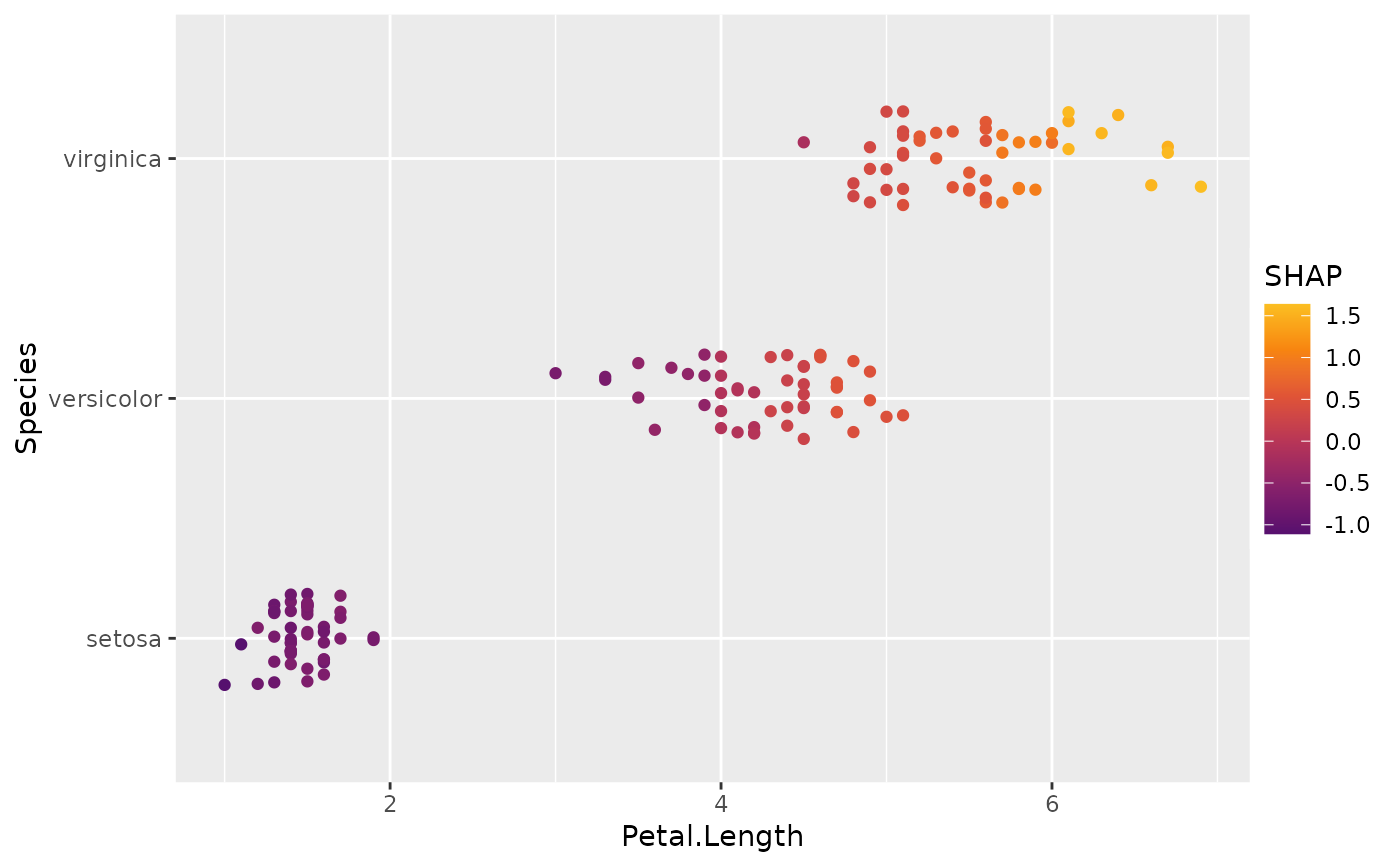
sv_dependence2D(sv, x = "Petal.Length", y = "Species")
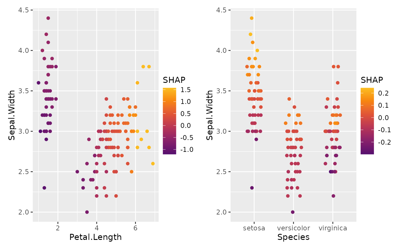
 sv_dependence2D(sv, x = c("Petal.Length", "Species"), y = "Sepal.Width")
 # SHAP interaction values
sv2 <- shapviz(fit, X_pred = dtrain, X = iris, interactions = TRUE)
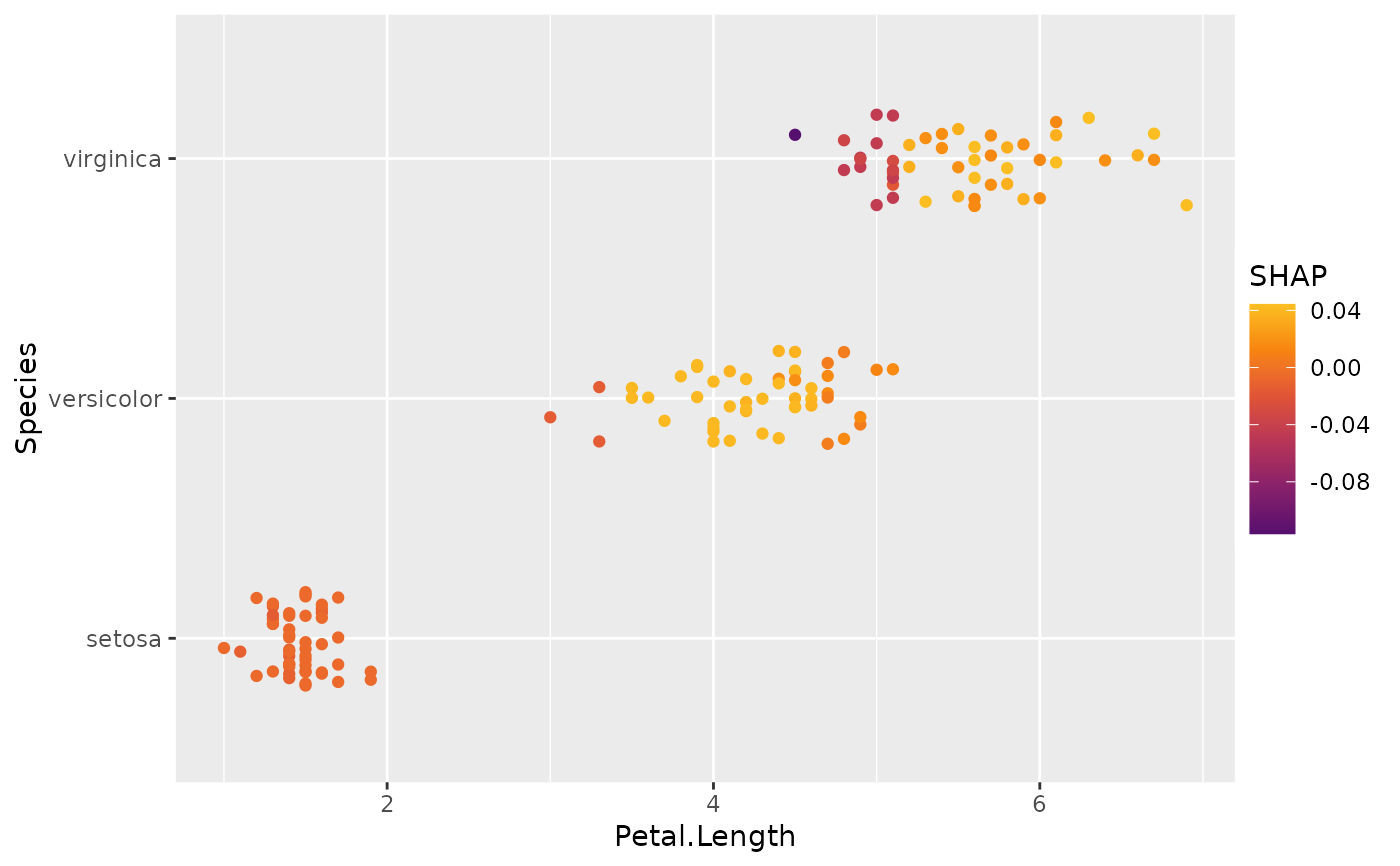
sv_dependence2D(sv2, x = "Petal.Length", y = "Species", interactions = TRUE)
# SHAP interaction values
sv2 <- shapviz(fit, X_pred = dtrain, X = iris, interactions = TRUE)
sv_dependence2D(sv2, x = "Petal.Length", y = "Species", interactions = TRUE)
 sv_dependence2D(
sv2,
x = "Petal.Length", y = c("Species", "Petal.Width"), interactions = TRUE
)
sv_dependence2D(
sv2,
x = "Petal.Length", y = c("Species", "Petal.Width"), interactions = TRUE
)
 # mshapviz object
mx <- split(sv, f = iris$Species)
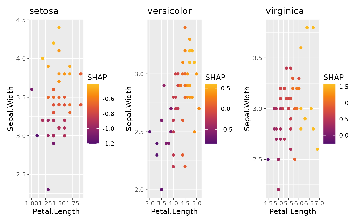
sv_dependence2D(mx, x = "Petal.Length", y = "Sepal.Width")
# mshapviz object
mx <- split(sv, f = iris$Species)
sv_dependence2D(mx, x = "Petal.Length", y = "Sepal.Width")