How to use multilabel classification and DALEX?
Szymon Maksymiuk
2023-03-22
Source:vignettes/multilabel_classification.Rmd
multilabel_classification.RmdData for HR example
In the following vignette, we will walk through a multilabel
classification example with DALEX. The purpose of this
tutorial is that for some of DALEX functionalities binary
classification is a default one, and therefore we need to put some
self-made code to work here. All of the examples will be performed with
HR dataset that is available in DALEX, it’s
target column is status with three-level factor. For all
cases our model will be ranger.
library("DALEX")
old_theme = set_theme_dalex("ema")

data(HR)
head(HR)
#> gender age hours evaluation salary status
#> 1 male 32.58267 41.88626 3 1 fired
#> 2 female 41.21104 36.34339 2 5 fired
#> 3 male 37.70516 36.81718 3 0 fired
#> 4 female 30.06051 38.96032 3 2 fired
#> 5 male 21.10283 62.15464 5 3 promoted
#> 6 male 40.11812 69.53973 2 0 firedCreation of model and explainer
Ok, now it is time to create a model.
library("ranger")
model_HR_ranger <- ranger(status~.,  data = HR, probability = TRUE, num.trees = 50)
model_HR_ranger
#> Ranger result
#>
#> Call:
#> ranger(status ~ ., data = HR, probability = TRUE, num.trees = 50)
#>
#> Type: Probability estimation
#> Number of trees: 50
#> Sample size: 7847
#> Number of independent variables: 5
#> Mtry: 2
#> Target node size: 10
#> Variable importance mode: none
#> Splitrule: gini
#> OOB prediction error (Brier s.): 0.2177127
library("DALEX")
explain_HR_ranger <- explain(model_HR_ranger,
                              data = HR[,-6],
                              y = HR$status,
                              label = "Ranger Multilabel Classification",
                              colorize = FALSE)
#> Preparation of a new explainer is initiated
#> -> model label : Ranger Multilabel Classification
#> -> data : 7847 rows 5 cols
#> -> target variable : 7847 values
#> -> predict function : yhat.ranger will be used ( default )
#> -> predicted values : No value for predict function target column. ( default )
#> -> model_info : package ranger , ver. 0.14.1 , task multiclass ( default )
#> -> predicted values : predict function returns multiple columns: 3 ( default )
#> -> residual function : difference between 1 and probability of true class ( default )
#> -> residuals : numerical, min = 0 , mean = 0.2737901 , max = 0.9191974
#> A new explainer has been created!The sixth column, that we have omitted during the creation of the
explainer, stands for the target column (status). It is
good practice not to put it in data. Keep in mind that the
default yhat function for ranger, and for any
other package that is supported by DALEX, enforces
probability output. Therefore residuals cannot be standard \(y - \hat{y}\). Since
DALEX 1.2.2 in the case of multiclass classification one
minus probability of the TRUE class is a standard residual function.
Model Parts
In order to use model_parts() (former
variable_importance()) function it is necessary to switch
default loss_function argument to one that handle multiple
classes. DALEX has implemented one function like that and
it is called loss_cross_entropy(). To use it,
y parameter passed to explain function should
have exactly the same format as the target vector used for the training
process (ie. the same number of levels and names of those levels).
Also, we need probability outputs so there is no need to change the
default predict_function parameter.
library("DALEX")
explain_HR_ranger_new_y <- explain(model_HR_ranger,
                              data = HR[,-6],
                              y = HR$status,
                              label = "Ranger Multilabel Classification",
                              colorize = FALSE)
#> Preparation of a new explainer is initiated
#> -> model label : Ranger Multilabel Classification
#> -> data : 7847 rows 5 cols
#> -> target variable : 7847 values
#> -> predict function : yhat.ranger will be used ( default )
#> -> predicted values : No value for predict function target column. ( default )
#> -> model_info : package ranger , ver. 0.14.1 , task multiclass ( default )
#> -> predicted values : predict function returns multiple columns: 3 ( default )
#> -> residual function : difference between 1 and probability of true class ( default )
#> -> residuals : numerical, min = 0 , mean = 0.2737901 , max = 0.9191974
#> A new explainer has been created!And now we can use model_parts()
mp <- model_parts(explain_HR_ranger_new_y, loss_function = loss_cross_entropy)
plot(mp)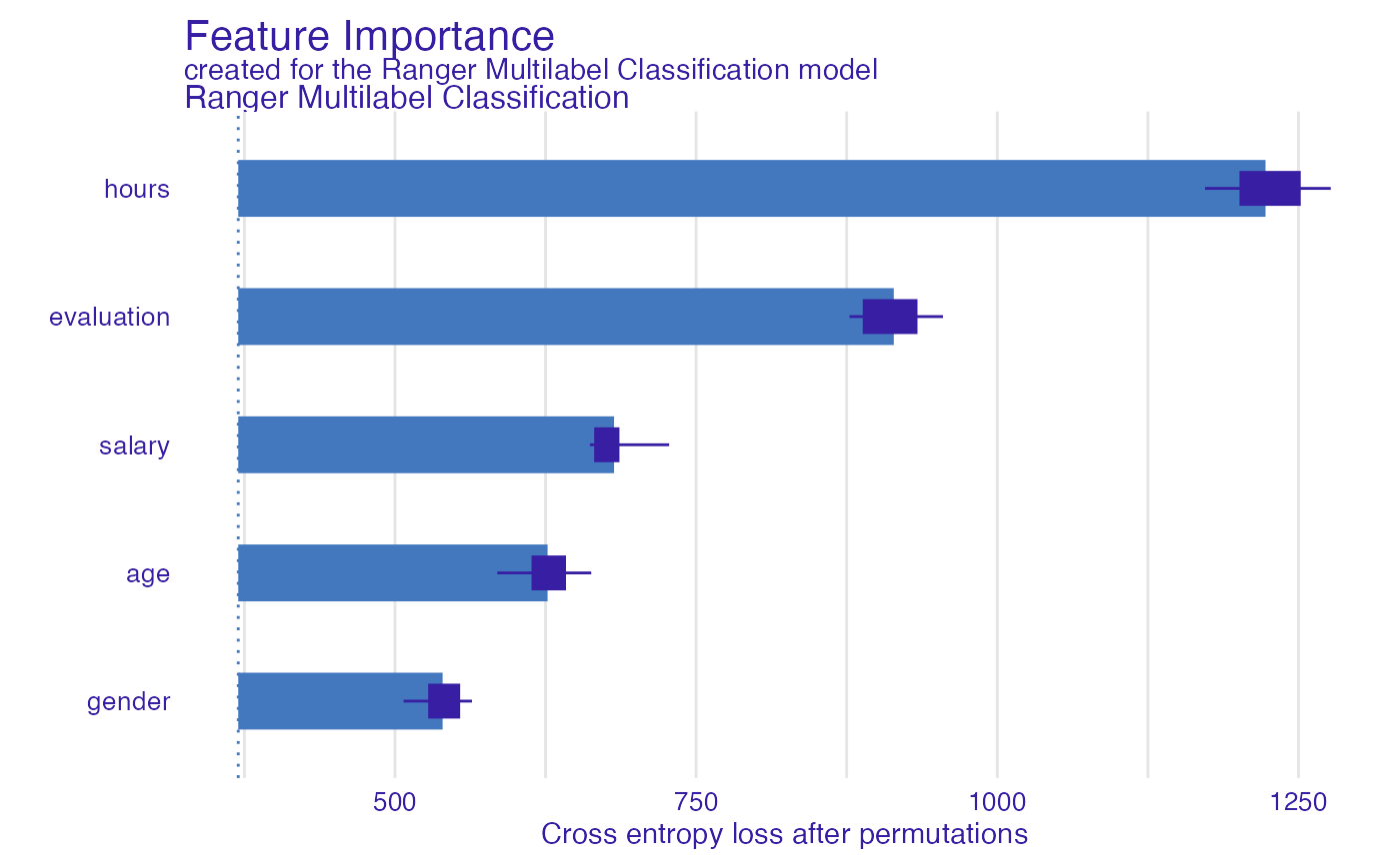
As we see above, we can enjoy perfectly fine variable importance plot.
Model Profile
There is no need for tricks in order to use
model_profile() (former variable_effect()).
Our target will be one-hot-encoded, and all of the explanations will be
performed for each of class separately.
partial_dependency
mp_p <- model_profile(explain_HR_ranger, variables = "salary", type = "partial")
mp_p$color <- "_label_"
plot(mp_p)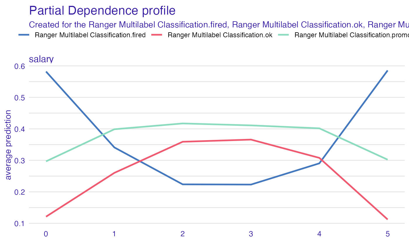
accumulated_dependency
mp_a <- model_profile(explain_HR_ranger, variables = "salary", type = "accumulated")
mp_a$color = "_label_"
plot(mp_a)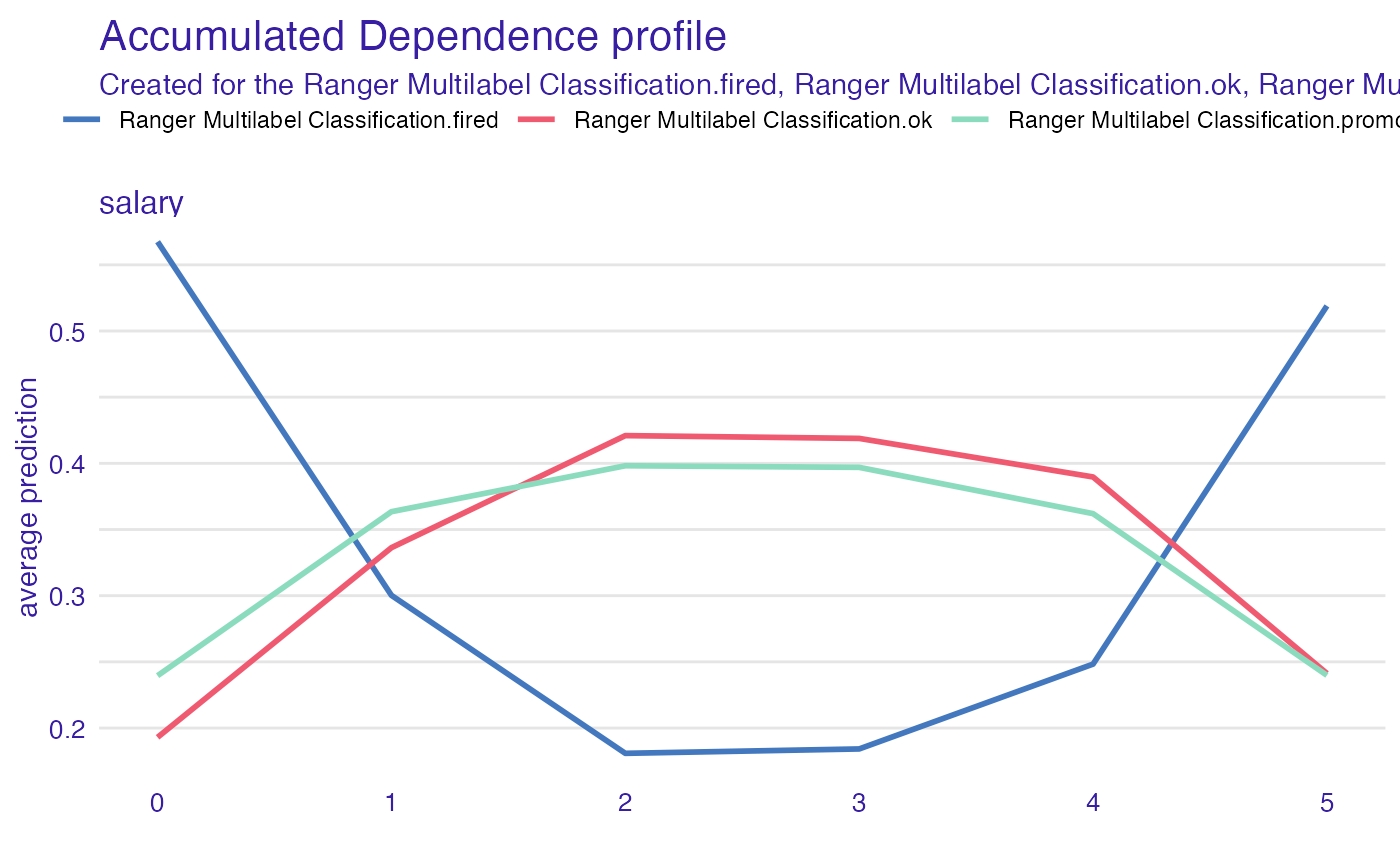
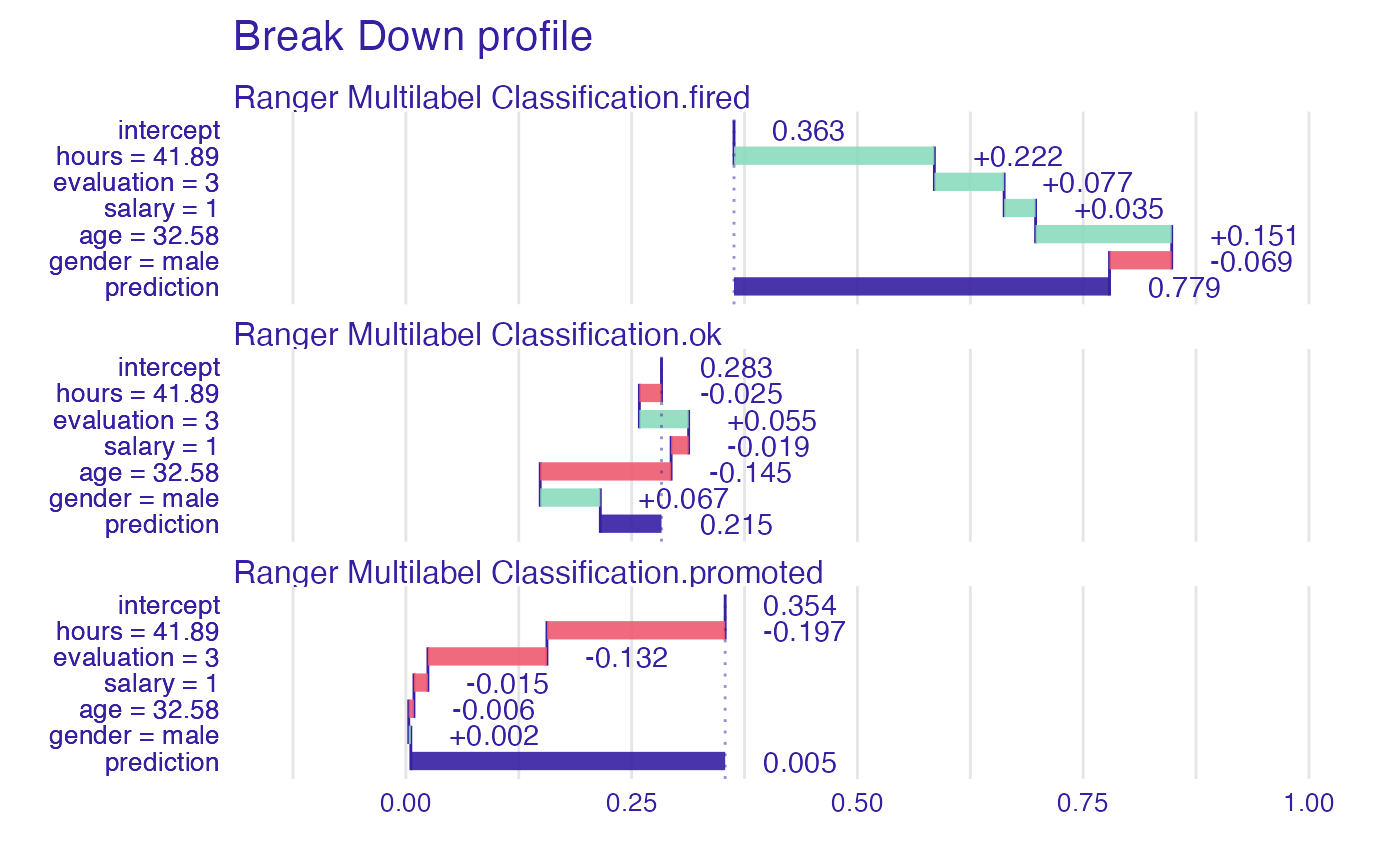
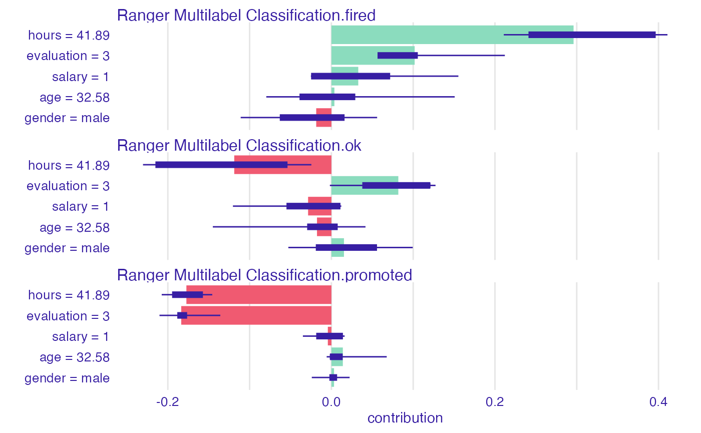
Instance level explanations
As above, predict_parts() (former
variable_attribution()) works perfectly fine with
multilabel classification and default explainer. Just like before, our
target will be split into variables standing for each factor level and
computations will be performed then.
model_performance and predict_diagnostics
The description of those two functions is merged into one paragraph
because they require the same action to get them to work with multilabel
classification. The most important thing here is to realize that both
functions are based on residuals. Since DALEX 1.2.2,
explain function recognizes if a model is a multiclass classification
task and uses a dedicated residual function as default.
Model Performance
(mp <- model_performance(explain_HR_ranger))#> Measures for: multiclass
#> micro_F1 : 0.8724353
#> macro_F1 : 0.8706813
#> w_macro_F1 : 0.8713967
#> accuracy : 0.8724353
#> w_macro_auc: 0.9778784
#> cross_entro: 2930.612
#>
#> Residuals:
#> 0% 10% 20% 30% 40% 50% 60%
#> 0.00000000 0.02225074 0.05952983 0.11272423 0.17004446 0.23497789 0.30970797
#> 70% 80% 90% 100%
#> 0.39054829 0.47851959 0.58846512 0.91919737
plot(mp)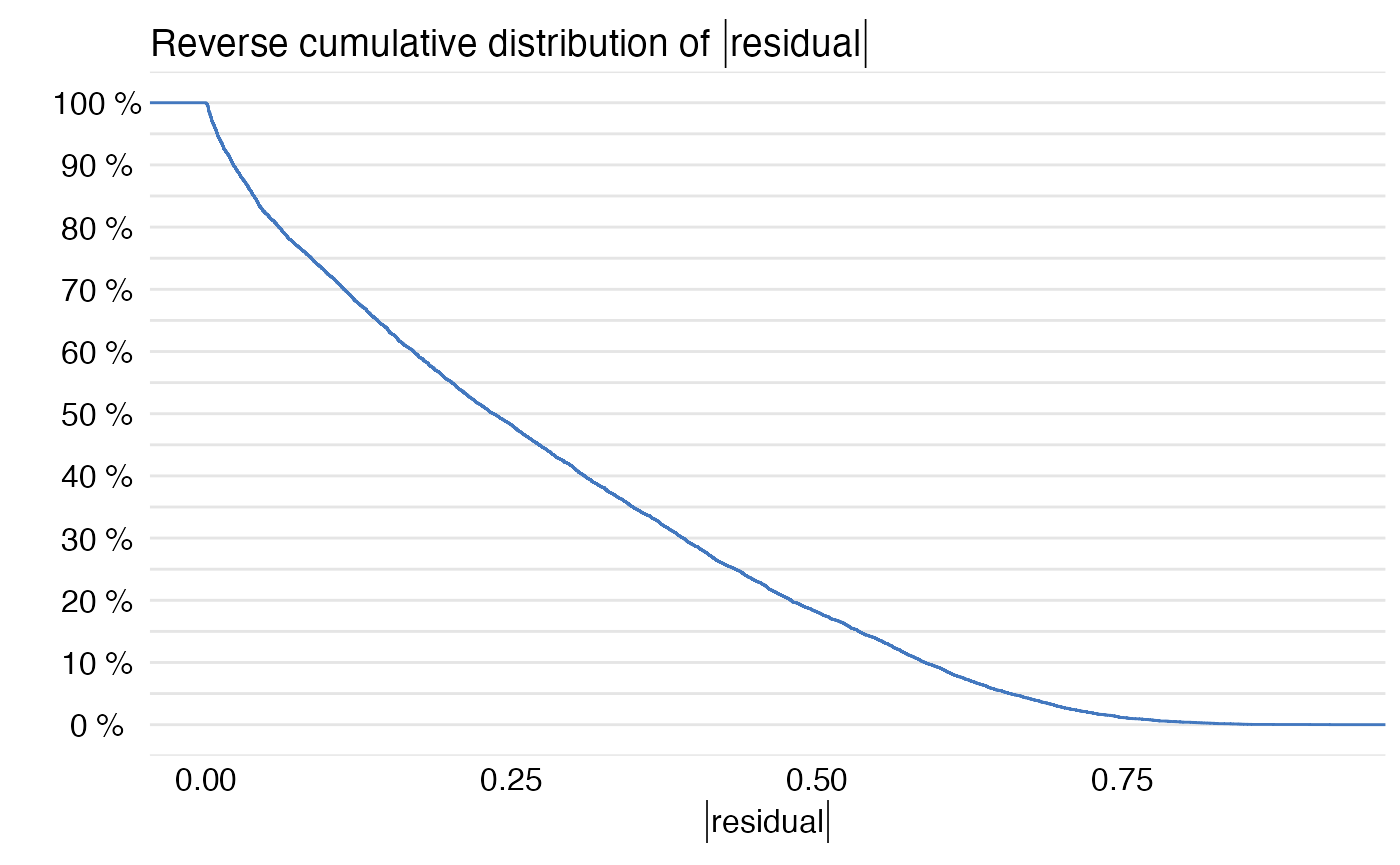
Predict diagnostics
pd_all <- predict_diagnostics(explain_HR_ranger, HR[1,])
plot(pd_all)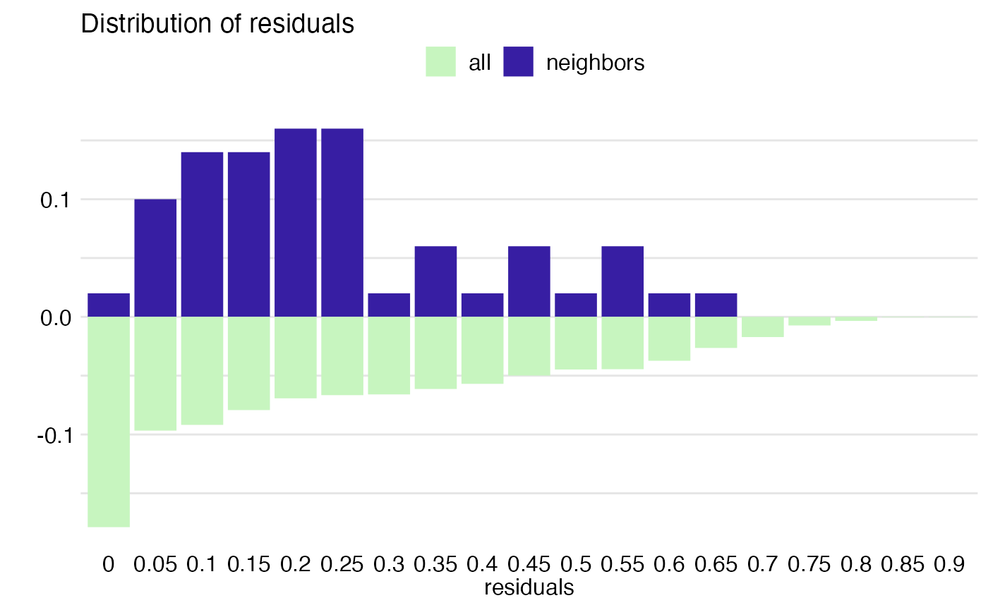
pd_salary <- predict_diagnostics(explain_HR_ranger, HR[1,], variables = "salary")
plot(pd_salary)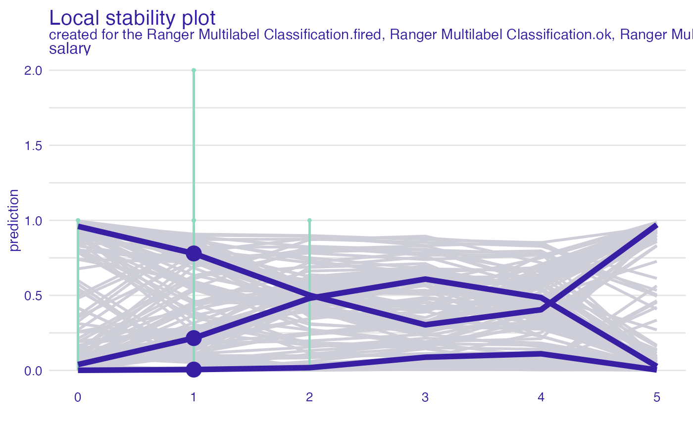
Session info
#> R version 4.2.3 (2023-03-15)
#> Platform: x86_64-apple-darwin17.0 (64-bit)
#> Running under: macOS Big Sur ... 10.16
#>
#> Matrix products: default
#> BLAS:   /Library/Frameworks/R.framework/Versions/4.2/Resources/lib/libRblas.0.dylib
#> LAPACK: /Library/Frameworks/R.framework/Versions/4.2/Resources/lib/libRlapack.dylib
#>
#> locale:
#> [1] en_US.UTF-8/en_US.UTF-8/en_US.UTF-8/C/en_US.UTF-8/en_US.UTF-8
#>
#> attached base packages:
#> [1] stats     graphics  grDevices utils     datasets  methods   base
#>
#> other attached packages:
#> [1] ranger_0.14.1 DALEX_2.5.1
#>
#> loaded via a namespace (and not attached):
#>  [1] tidyselect_1.2.0  xfun_0.37         bslib_0.4.2       purrr_1.0.1
#>  [5] lattice_0.20-45   colorspace_2.1-0  vctrs_0.6.1       generics_0.1.3
#>  [9] htmltools_0.5.4   yaml_2.3.7        utf8_1.2.3        rlang_1.1.0
#> [13] pkgdown_2.0.7     jquerylib_0.1.4   pillar_1.9.0      glue_1.6.2
#> [17] withr_2.5.0       lifecycle_1.0.3   stringr_1.5.0     munsell_0.5.0
#> [21] gtable_0.3.3      ragg_1.2.5        memoise_2.0.1     evaluate_0.20
#> [25] labeling_0.4.2    knitr_1.42        fastmap_1.1.1     fansi_1.0.4
#> [29] highr_0.10        iBreakDown_2.0.1  Rcpp_1.0.10       scales_1.2.1
#> [33] cachem_1.0.7      desc_1.4.2        jsonlite_1.8.4    ingredients_2.3.0
#> [37] farver_2.1.1      systemfonts_1.0.4 fs_1.6.1          textshaping_0.3.6
#> [41] ggplot2_3.4.1     digest_0.6.31     stringi_1.7.12    dplyr_1.1.1
#> [45] grid_4.2.3        rprojroot_2.0.3   cli_3.6.0         tools_4.2.3
#> [49] magrittr_2.0.3    sass_0.4.5        tibble_3.2.1      pkgconfig_2.0.3
#> [53] Matrix_1.5-3      gower_1.0.1       rmarkdown_2.20    R6_2.5.1
#> [57] compiler_4.2.3