How to use DALEX with the yardstick package?
Przemyslaw Biecek
2023-03-22
Source:vignettes/vignette_yardstick.Rmd
vignette_yardstick.RmdIntro
yardstick
is a package that offers many measures for evaluating model performance.
It is based on the tidymodels/tidyverse
philosophy, the performance is calculated by functions working on the
data.frame with the results of the model.
DALEX uses model performance
measures to assess the importance of variables (in the model_parts
function). These are typically calculated based on loss functions
(functions with prefix loss) that are working on two
vectors - the score from the model and the true target variable.
Although these packages have a slightly different philosophy of
operation, you can use the measures available in yardstick when working
with DALEX. Below is information on how to use the
loss_yardstick function to do this.
Prepare a classification model
The yardstick package supports both classification
models and regression models. We will start our example with a
classification model for the titanic data - the probability of surviving
this disaster.
The following instruction trains a classification model.
library("DALEX")
library("yardstick")
titanic_glm <- glm(survived~., data = titanic_imputed, family = "binomial")
Class Probability Metrics
The Class Probability Metrics in the yardstick package
assume that the true value is a factor and the model
returns a numerical score. So let’s prepare an explainer
that has factor as y and the
predict_function returns the probability of the target
class (default behaviour).
NOTE: Performance measures will be calculated on data supplied in the explainer. Put here the test data!
explainer_glm <- DALEX::explain(titanic_glm,
                        data = titanic_imputed[,-8],
                        y = factor(titanic_imputed$survived))
To make functions from the yardstick compatible with
DALEX we must use the loss_yardstick adapter.
In the example below we use the roc_auc function (area
under the receiver operator curve). The yardstick:: prefix
is not necessary, but we put it here to show explicitly where the
functions you use are located.
NOTE: we set
yardstick.event_first = FALSE as the model predicts
probability of survived = 1.
options(yardstick.event_first = FALSE)

glm_auc <- model_parts(explainer_glm, type = "raw",
                  loss_function = loss_yardstick(yardstick::roc_auc))
glm_auc
#> variable mean_dropout_loss label
#> 1 _full_model_ 0.8089452 lm
#> 2 gender 0.6238639 lm
#> 3 class 0.7099712 lm
#> 4 age 0.7813811 lm
#> 5 sibsp 0.7995240 lm
#> 6 embarked 0.8027081 lm
#> 7 parch 0.8089237 lm
#> 8 fare 0.8095338 lm
#> 9 _baseline_ 0.4990260 lm
plot(glm_auc)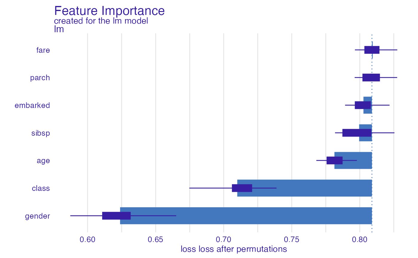
In a similar way, we can use the pr_auc function (area
under the precision recall curve).
glm_prauc <- model_parts(explainer_glm, type = "raw",
                  loss_function = loss_yardstick(yardstick::pr_auc))
glm_prauc
#> variable mean_dropout_loss label
#> 1 _full_model_ 0.7426051 lm
#> 2 gender 0.4370993 lm
#> 3 class 0.5874661 lm
#> 4 age 0.7246998 lm
#> 5 sibsp 0.7264267 lm
#> 6 embarked 0.7322981 lm
#> 7 fare 0.7417359 lm
#> 8 parch 0.7422524 lm
#> 9 _baseline_ 0.3259686 lm
plot(glm_prauc)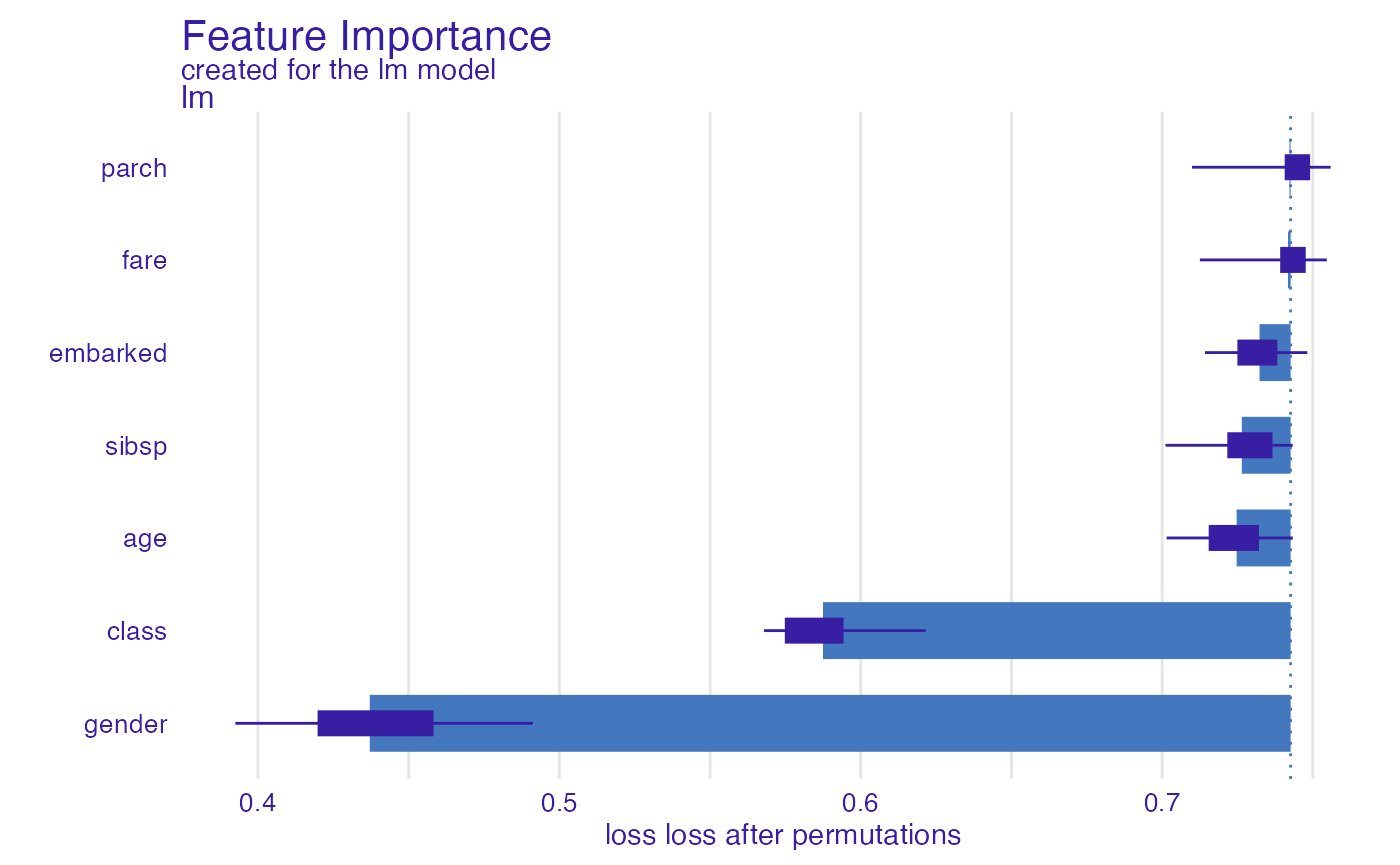
Classification Metrics
The Classification Metrics in the yardstick package
assume that the true value is a factor and the model
returns a factor variable.
This is different behavior than for most explanations in DALEX, because when explaining predictions we typically operate on class membership probabilities. If we want to use Classification Metrics we need to provide a predict function that returns classes instead of probabilities.
So let’s prepare an explainer that has
factor as y and the
predict_function returns classes.
explainer_glm <- DALEX::explain(titanic_glm,
                        data = titanic_imputed[,-8],
                        y = factor(titanic_imputed$survived),
                        predict_function = function(m,x) {
                              factor(as.numeric(predict(m, x, type = "response") > 0.5),
                                     levels = c("0", "1"))
                        })
Again, let’s use the loss_yardstick adapter. In the
example below we use the accuracy function.
glm_accuracy <- model_parts(explainer_glm, type = "raw",
                    loss_function = loss_yardstick(yardstick::accuracy))
glm_accuracy
#> variable mean_dropout_loss label
#> 1 _full_model_ 0.7978 lm
#> 2 gender 0.6369 lm
#> 3 class 0.7454 lm
#> 4 age 0.7819 lm
#> 5 sibsp 0.7914 lm
#> 6 embarked 0.7957 lm
#> 7 parch 0.7971 lm
#> 8 fare 0.7980 lm
#> 9 _baseline_ 0.5894 lm
plot(glm_accuracy)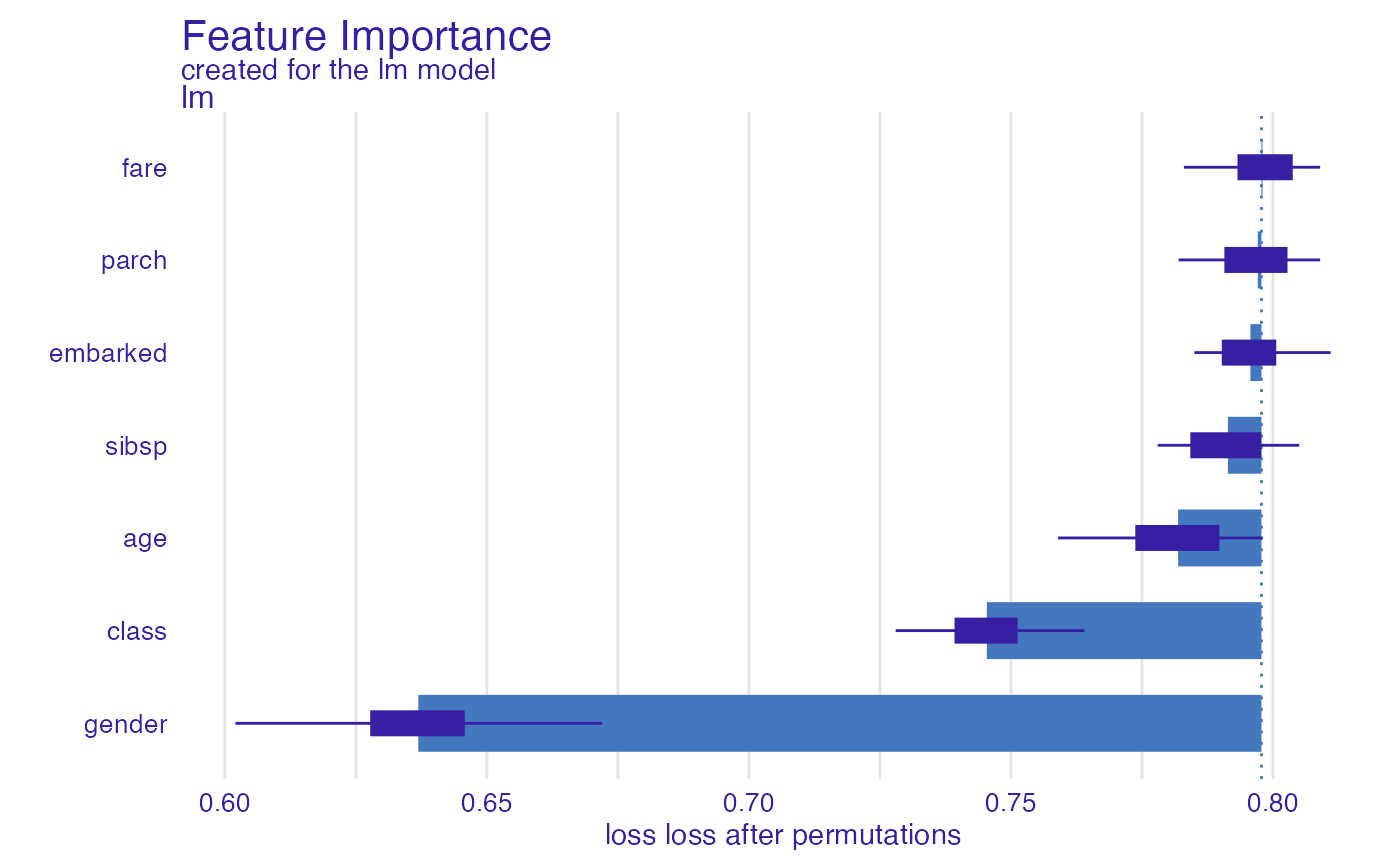
In a similar way, we can use the bal_accuracy function
(balanced accuracy).
glm_bal_accuracy <- model_parts(explainer_glm, type = "raw",
                    loss_function = loss_yardstick(yardstick::bal_accuracy))
glm_bal_accuracy
#> variable mean_dropout_loss label
#> 1 _full_model_ 0.7419681 lm
#> 2 gender 0.5716828 lm
#> 3 class 0.6715899 lm
#> 4 age 0.7263103 lm
#> 5 embarked 0.7361306 lm
#> 6 sibsp 0.7389633 lm
#> 7 fare 0.7413686 lm
#> 8 parch 0.7419721 lm
#> 9 _baseline_ 0.4997630 lm
plot(glm_bal_accuracy)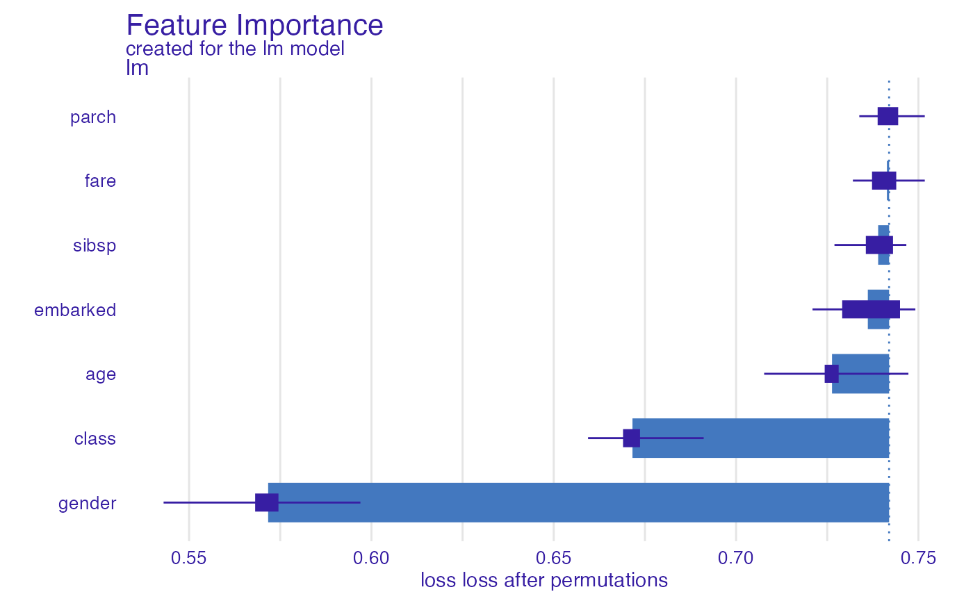
The lower the better?
For the loss function, the smaller the values the better the model.
Therefore, the importance of variables is often calculated as
loss(perturbed) - loss(original).
But many model performance functions have the opposite
characteristic, the higher they are the better (e.g. AUC,
accuracy, etc). To maintain a consistent analysis pipeline
it is convenient to invert such functions, e.g. by converting to
1- AUC or 1 - accuracy.
To do it, just add the reverse = TRUE argument.
glm_1accuracy <- model_parts(explainer_glm,
                    loss_function = loss_yardstick(accuracy, reverse = TRUE))
glm_1accuracy
#> variable mean_dropout_loss label
#> 1 _full_model_ 0.2043 lm
#> 2 fare 0.2042 lm
#> 3 parch 0.2046 lm
#> 4 embarked 0.2083 lm
#> 5 sibsp 0.2106 lm
#> 6 age 0.2194 lm
#> 7 class 0.2614 lm
#> 8 gender 0.3694 lm
#> 9 _baseline_ 0.4071 lm
plot(glm_1accuracy)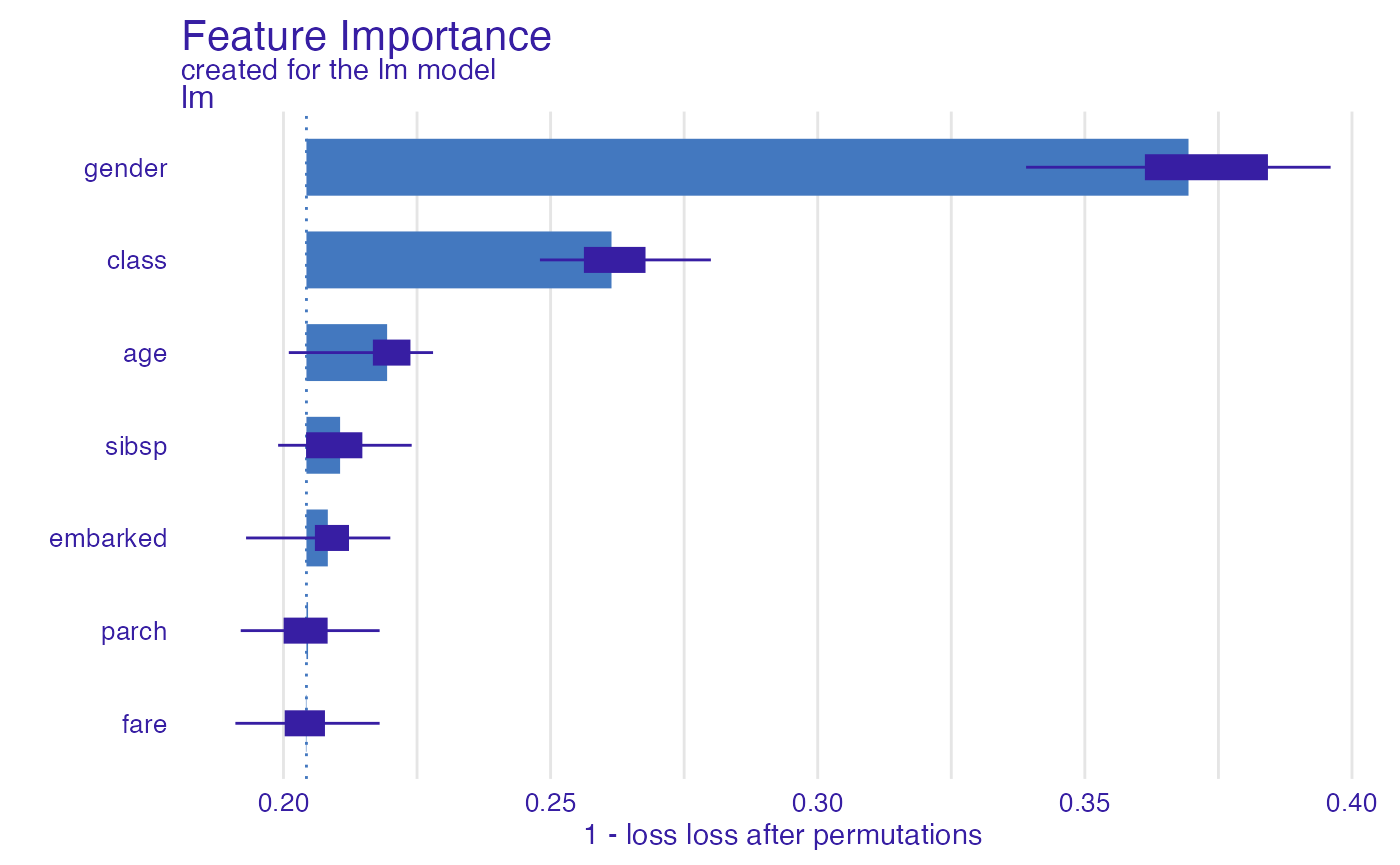
Calculate performance on whole dataset
By default the performance is calculated on N = 1000
randomly selected observations (to speed up the calculations). Set
N = NULL to use the whole dataset.
glm_1accuracy <- model_parts(explainer_glm,
                    loss_function = loss_yardstick(accuracy, reverse = TRUE),
                    N = NULL)
plot(glm_1accuracy)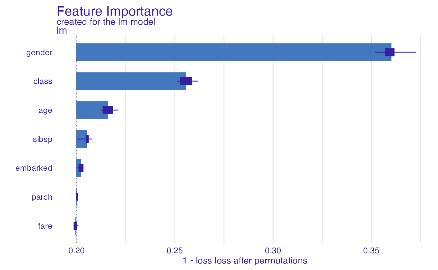
Prepare a regression model
The following instruction trains a regression model.
Regression Metrics
The Regression Metrics in the yardstick package assume
that the true value is a numeric variable and the model
returns a numeric score.
explainer_ranger  <- DALEX::explain(apartments_ranger, data = apartments[,-1],
                             y = apartments$m2.price, label = "Ranger Apartments")
#> Preparation of a new explainer is initiated
#> -> model label : Ranger Apartments
#> -> data : 1000 rows 5 cols
#> -> target variable : 1000 values
#> -> predict function : yhat.ranger will be used ( default )
#> -> predicted values : No value for predict function target column. ( default )
#> -> model_info : package ranger , ver. 0.14.1 , task regression ( default )
#> -> predicted values : numerical, min = 1907.767 , mean = 3488.795 , max = 6181.198
#> -> residual function : difference between y and yhat ( default )
#> -> residuals : numerical, min = -643.31 , mean = -1.775808 , max = 708.0153
#> A new explainer has been created!To make functions from the yardstick compatible with
DALEX we must use the loss_yardstick adapter.
In the example below we use the rmse function (root mean
squared error).
ranger_rmse <- model_parts(explainer_ranger, type = "raw",
                      loss_function = loss_yardstick(rmse))
ranger_rmse
#> variable mean_dropout_loss label
#> 1 _full_model_ 166.5718 Ranger Apartments
#> 2 no.rooms 320.9772 Ranger Apartments
#> 3 construction.year 394.2647 Ranger Apartments
#> 4 floor 442.0134 Ranger Apartments
#> 5 surface 541.2952 Ranger Apartments
#> 6 district 739.4888 Ranger Apartments
#> 7 _baseline_ 1205.0356 Ranger Apartments
plot(ranger_rmse)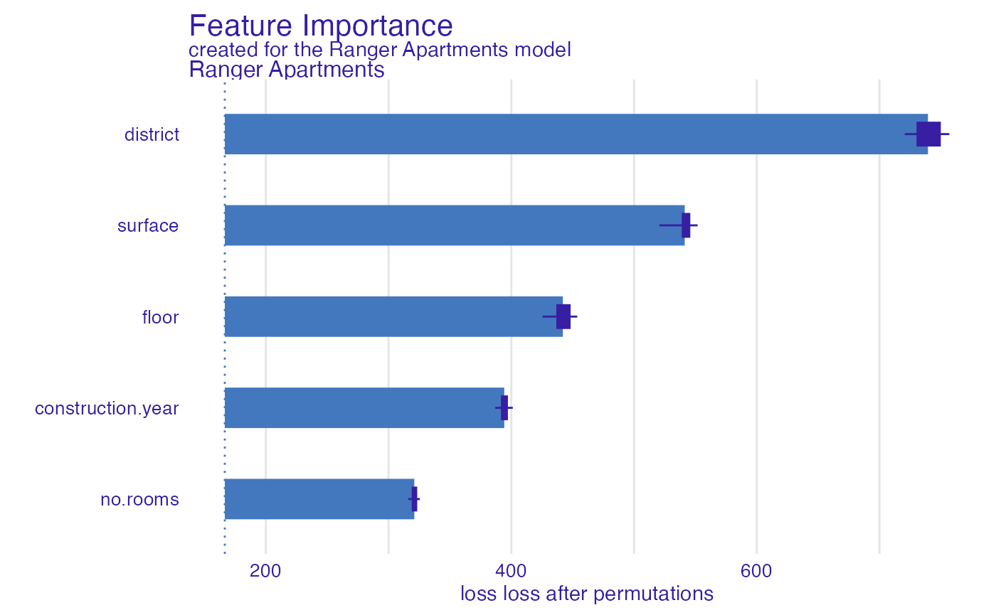
And one more example for rsq function (R squared).
ranger_rsq <- model_parts(explainer_ranger, type = "raw",
                      loss_function = loss_yardstick(rsq))
ranger_rsq
#> variable mean_dropout_loss label
#> 1 _full_model_ 0.979198764 Ranger Apartments
#> 2 district 0.352448580 Ranger Apartments
#> 3 surface 0.650201959 Ranger Apartments
#> 4 floor 0.764333307 Ranger Apartments
#> 5 construction.year 0.821802873 Ranger Apartments
#> 6 no.rooms 0.922314139 Ranger Apartments
#> 7 _baseline_ 0.000930641 Ranger Apartments
plot(ranger_rsq)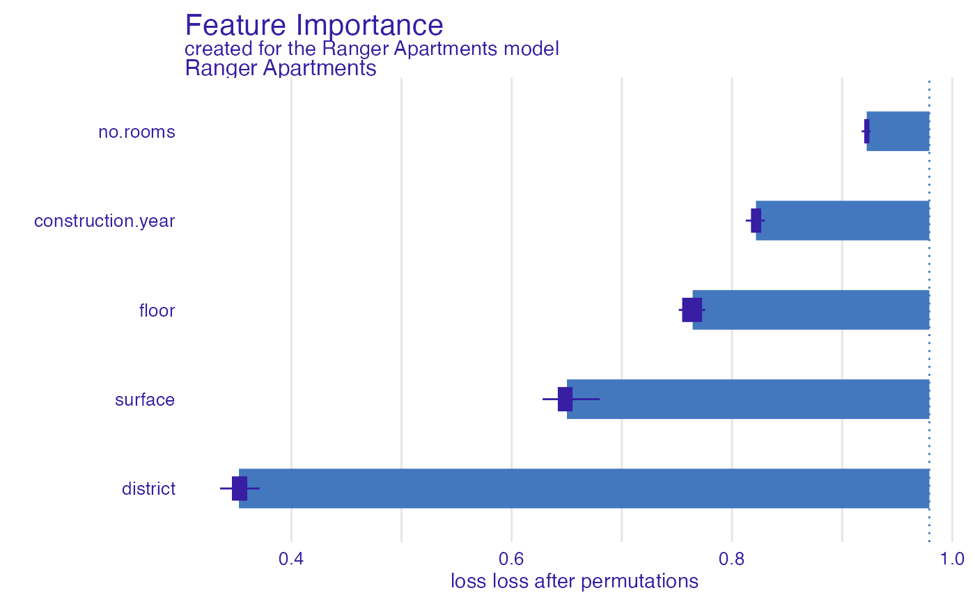
Summary
I hope that using the yardstick package at
DALEX will now be easy and enjoyable. If you would like to
share your experience with this package, please create an issue at https://github.com/ModelOriented/DALEX/issues.
Session info
#> R version 4.2.3 (2023-03-15)
#> Platform: x86_64-apple-darwin17.0 (64-bit)
#> Running under: macOS Big Sur ... 10.16
#>
#> Matrix products: default
#> BLAS:   /Library/Frameworks/R.framework/Versions/4.2/Resources/lib/libRblas.0.dylib
#> LAPACK: /Library/Frameworks/R.framework/Versions/4.2/Resources/lib/libRlapack.dylib
#>
#> locale:
#> [1] en_US.UTF-8/en_US.UTF-8/en_US.UTF-8/C/en_US.UTF-8/en_US.UTF-8
#>
#> attached base packages:
#> [1] stats     graphics  grDevices utils     datasets  methods   base
#>
#> other attached packages:
#> [1] ranger_0.14.1   yardstick_1.1.0 DALEX_2.5.1
#>
#> loaded via a namespace (and not attached):
#>  [1] tidyselect_1.2.0  xfun_0.37         bslib_0.4.2       purrr_1.0.1
#>  [5] lattice_0.20-45   colorspace_2.1-0  vctrs_0.6.1       generics_0.1.3
#>  [9] htmltools_0.5.4   yaml_2.3.7        utf8_1.2.3        rlang_1.1.0
#> [13] pkgdown_2.0.7     jquerylib_0.1.4   pillar_1.9.0      glue_1.6.2
#> [17] withr_2.5.0       lifecycle_1.0.3   stringr_1.5.0     munsell_0.5.0
#> [21] gtable_0.3.3      ragg_1.2.5        memoise_2.0.1     evaluate_0.20
#> [25] labeling_0.4.2    knitr_1.42        fastmap_1.1.1     fansi_1.0.4
#> [29] highr_0.10        Rcpp_1.0.10       scales_1.2.1      cachem_1.0.7
#> [33] desc_1.4.2        jsonlite_1.8.4    ingredients_2.3.0 farver_2.1.1
#> [37] systemfonts_1.0.4 fs_1.6.1          textshaping_0.3.6 ggplot2_3.4.1
#> [41] digest_0.6.31     stringi_1.7.12    dplyr_1.1.1       grid_4.2.3
#> [45] rprojroot_2.0.3   cli_3.6.0         tools_4.2.3       magrittr_2.0.3
#> [49] sass_0.4.5        tibble_3.2.1      crayon_1.5.2      pkgconfig_2.0.3
#> [53] Matrix_1.5-3      rmarkdown_2.20    R6_2.5.1          compiler_4.2.3