Survival on the RMS Titanic

Data for Titanic survival

Let’s see an example for DALEX package for classification models for the survival problem for Titanic dataset. Here we are using a dataset titanic available in the DALEX package. Note that this data was copied from the stablelearner package.

library("DALEX")
head(titanic_imputed)

#>   gender age class    embarked  fare sibsp parch survived
#> 1   male  42   3rd Southampton  7.11     0     0        0
#> 2   male  13   3rd Southampton 20.05     0     2        0
#> 3   male  16   3rd Southampton 20.05     1     1        0
#> 4 female  39   3rd Southampton 20.05     1     1        1
#> 5 female  16   3rd Southampton  7.13     0     0        1
#> 6   male  25   3rd Southampton  7.13     0     0        1

Model for Titanic survival

Ok, not it’s time to create a model. Let’s use the Random Forest model.

# prepare model
library("ranger")
model_titanic_rf <- ranger(survived ~ gender + age + class + embarked +
                                   fare + sibsp + parch,  data = titanic_imputed,
                           classification = TRUE)
model_titanic_rf

#> Ranger result
#> 
#> Call:
#>  ranger(survived ~ gender + age + class + embarked + fare + sibsp +      parch, data = titanic_imputed, classification = TRUE) 
#> 
#> Type:                             Classification 
#> Number of trees:                  500 
#> Sample size:                      2207 
#> Number of independent variables:  7 
#> Mtry:                             2 
#> Target node size:                 1 
#> Variable importance mode:         none 
#> Splitrule:                        gini 
#> OOB prediction error:             20.03 %

Explainer for Titanic survival

The third step (it’s optional but useful) is to create a DALEX explainer for the random forest model.

library("DALEX")
explain_titanic_rf <- explain(model_titanic_rf, 
                      data = titanic_imputed,
                      y = titanic_imputed$survived, 
                      label = "Random Forest v7",
                      colorize = FALSE)

#> Preparation of a new explainer is initiated
#>   -> model label       :  Random Forest v7 
#>   -> data              :  2207  rows  8  cols 
#>   -> target variable   :  2207  values 
#>   -> predict function  :  yhat.ranger  will be used (  default  )
#>   -> predicted values  :  No value for predict function target column. (  default  )
#>   -> model_info        :  package ranger , ver. 0.14.1 , task classification (  default  ) 
#>   -> predicted values  :  numerical, min =  0 , mean =  0.213865 , max =  1  
#>   -> residual function :  difference between y and yhat (  default  )
#>   -> residuals         :  numerical, min =  -1 , mean =  0.1082918 , max =  1  
#>   A new explainer has been created!

Variable importance plots

Use the variable_importance() explainer to present the importance of particular features. Note that type = "difference" normalizes dropouts, and now they all start in 0.

vi_rf <- model_parts(explain_titanic_rf)
head(vi_rf)

#>       variable mean_dropout_loss            label
#> 1 _full_model_         0.2164656 Random Forest v7
#> 2     survived         0.2164564 Random Forest v7
#> 3        parch         0.2309825 Random Forest v7
#> 4        sibsp         0.2360850 Random Forest v7
#> 5     embarked         0.2387941 Random Forest v7
#> 6         fare         0.2621238 Random Forest v7

plot(vi_rf)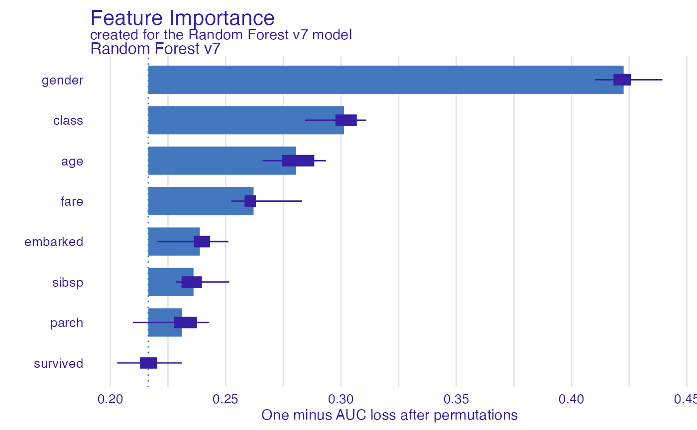

Variable effects

As we see the most important feature is Sex. Next three important features are Pclass, Age and Fare. Let’s see the link between model response and these features.

Such univariate relation can be calculated with variable_effect().

Age

Kids 5 years old and younger have a much higher survival probability.

vr_age  <- model_profile(explain_titanic_rf, variables =  "age")
head(vr_age)

#> $cp_profiles
#> Top profiles    : 
#>        gender        age            class    embarked fare sibsp parch survived
#> 2068     male  0.1666667 victualling crew Southampton    0     0     0        0
#> 2068.1   male  2.0000000 victualling crew Southampton    0     0     0        0
#> 2068.2   male  4.0000000 victualling crew Southampton    0     0     0        0
#> 2068.3   male  7.0000000 victualling crew Southampton    0     0     0        0
#> 2068.4   male  9.0000000 victualling crew Southampton    0     0     0        0
#> 2068.5   male 13.0000000 victualling crew Southampton    0     0     0        0
#>        _yhat_ _vname_ _ids_          _label_
#> 2068        0     age  2068 Random Forest v7
#> 2068.1      0     age  2068 Random Forest v7
#> 2068.2      0     age  2068 Random Forest v7
#> 2068.3      0     age  2068 Random Forest v7
#> 2068.4      0     age  2068 Random Forest v7
#> 2068.5      0     age  2068 Random Forest v7
#> 
#> 
#> Top observations:
#>      gender age            class    embarked    fare sibsp parch survived
#> 2068   male  33 victualling crew Southampton  0.0000     0     0        0
#> 689    male  38              3rd Southampton 56.0911     0     0        1
#> 886    male  41              3rd Southampton  7.0206     0     0        0
#> 1177   male  74              3rd Southampton  7.1506     0     0        0
#> 1871   male  42 victualling crew Southampton  0.0000     0     0        0
#> 957    male  21              3rd Southampton  7.1806     0     0        0
#>      _yhat_          _label_ _ids_
#> 2068      0 Random Forest v7     1
#> 689       1 Random Forest v7     2
#> 886       0 Random Forest v7     3
#> 1177      0 Random Forest v7     4
#> 1871      0 Random Forest v7     5
#> 957       0 Random Forest v7     6
#> 
#> $agr_profiles
#> Top profiles    : 
#>   _vname_          _label_        _x_ _yhat_ _ids_
#> 1     age Random Forest v7  0.1666667   0.50     0
#> 2     age Random Forest v7  2.0000000   0.56     0
#> 3     age Random Forest v7  4.0000000   0.56     0
#> 4     age Random Forest v7  7.0000000   0.49     0
#> 5     age Random Forest v7  9.0000000   0.40     0
#> 6     age Random Forest v7 13.0000000   0.19     0
#> 
#> $color
#> [1] "#4378bf"

plot(vr_age)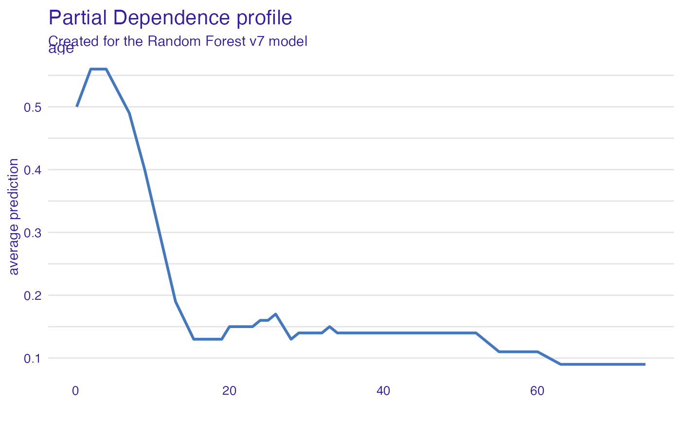

Passenger class

Passengers in the first-class have much higher survival probability.

vr_class  <- model_profile(explain_titanic_rf, variables =  "class")
plot(vr_class)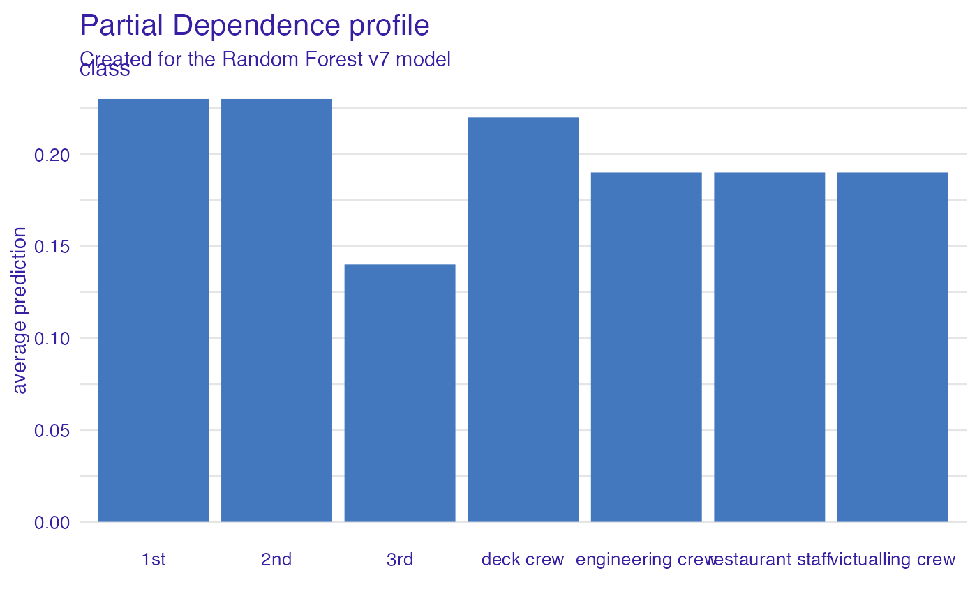

Fare

Very cheap tickets are linked with lower chances.

vr_fare  <- variable_profile(explain_titanic_rf, variables =  "fare")
plot(vr_fare)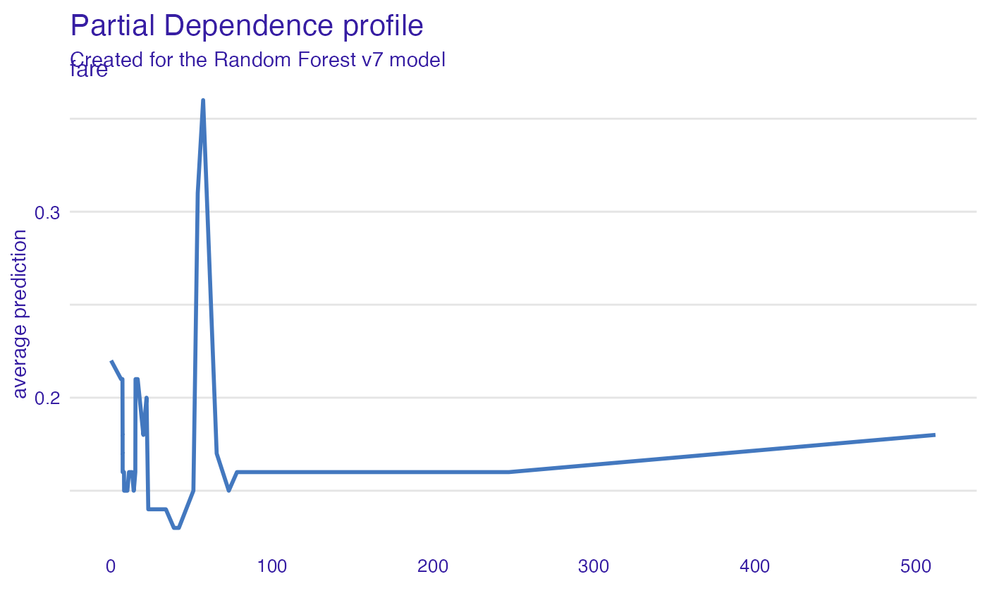

Embarked

Passengers that embarked from C have the highest survival.

vr_embarked  <- model_profile(explain_titanic_rf, variables =  "embarked")
plot(vr_embarked)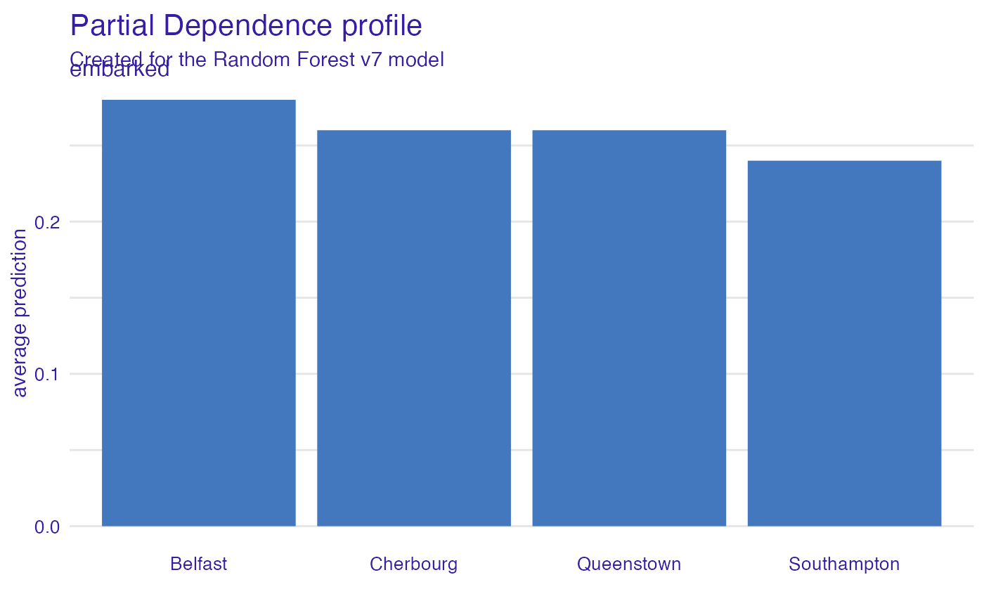

Instance level explanations

Let’s see break-down explanation for model predictions for 8 years old male from 1st class that embarked from port C.

new_passanger <- data.frame(
  class = factor("1st", levels = c("1st", "2nd", "3rd", "deck crew", "engineering crew", "restaurant staff", "victualling crew")),
  gender = factor("male", levels = c("female", "male")),
  age = 8,
  sibsp = 0,
  parch = 0,
  fare = 72,
  embarked = factor("Southampton", levels = c("Belfast", "Cherbourg", "Queenstown", "Southampton"))
)

sp_rf <- predict_parts(explain_titanic_rf, new_passanger)
plot(sp_rf)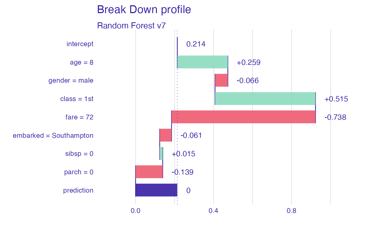

It looks like the most important feature for this passenger is age and sex. After all his odds for survival are higher than for the average passenger. Mainly because of the young age and despite being a male.

More models

Let’s train more models for survival.

Logistic regression

library("rms")
model_titanic_lmr <- lrm(survived ~ class + gender + rcs(age) + sibsp +
                   parch + fare + embarked, titanic_imputed)
explain_titanic_lmr <- explain(model_titanic_lmr, data = titanic_imputed, 
                   y = titanic_imputed$survived, 
                   predict_function = function(m,x) 
                            predict(m, x, type = "fitted"),
                   label = "Logistic regression")

#> Preparation of a new explainer is initiated
#>   -> model label       :  Logistic regression 
#>   -> data              :  2207  rows  8  cols 
#>   -> target variable   :  2207  values 
#>   -> predict function  :  function(m, x) predict(m, x, type = "fitted") 
#>   -> predicted values  :  No value for predict function target column. (  default  )
#>   -> model_info        :  package rms , ver. 6.5.0 , task classification (  default  ) 
#>   -> predicted values  :  numerical, min =  0.002671631 , mean =  0.3221568 , max =  0.9845724  
#>   -> residual function :  difference between y and yhat (  default  )
#>   -> residuals         :  numerical, min =  -0.9845724 , mean =  -2.491758e-09 , max =  0.9715125  
#>   A new explainer has been created!

Generalized Boosted Models (GBM)

library("gbm")
model_titanic_gbm <- gbm(survived  ~ class + gender + age + sibsp +
                     parch + fare + embarked, data = titanic_imputed, 
                     n.trees = 15000)

#> Distribution not specified, assuming bernoulli ...

explain_titanic_gbm <- explain(model_titanic_gbm, data = titanic_imputed, 
                       y = titanic_imputed$survived, 
                       predict_function = function(m,x) 
                            predict(m, x, n.trees = 15000, type = "response"),
                       label = "Generalized Boosted Models",
                       colorize = FALSE)

#> Preparation of a new explainer is initiated
#>   -> model label       :  Generalized Boosted Models 
#>   -> data              :  2207  rows  8  cols 
#>   -> target variable   :  2207  values 
#>   -> predict function  :  function(m, x) predict(m, x, n.trees = 15000, type = "response") 
#>   -> predicted values  :  No value for predict function target column. (  default  )
#>   -> model_info        :  package gbm , ver. 2.1.8.1 , task classification (  default  ) 
#>   -> predicted values  :  numerical, min =  0.0004911074 , mean =  0.3229161 , max =  0.9985837  
#>   -> residual function :  difference between y and yhat (  default  )
#>   -> residuals         :  numerical, min =  -0.9657513 , mean =  -0.0007592975 , max =  0.9865362  
#>   A new explainer has been created!

Support Vector Machines (SVM)

library("e1071")
model_titanic_svm <- svm(survived ~ class + gender + age + sibsp +
                     parch + fare + embarked, data = titanic_imputed, 
             type = "C-classification", probability = TRUE)
explain_titanic_svm <- explain(model_titanic_svm, data = titanic_imputed, 
                       y = titanic_imputed$survived, 
                       label = "Support Vector Machines",
                       colorize = FALSE)

#> Preparation of a new explainer is initiated
#>   -> model label       :  Support Vector Machines 
#>   -> data              :  2207  rows  8  cols 
#>   -> target variable   :  2207  values 
#>   -> predict function  :  yhat.svm  will be used (  default  )
#>   -> predicted values  :  No value for predict function target column. (  default  )
#>   -> model_info        :  package e1071 , ver. 1.7.13 , task classification (  default  ) 
#>   -> predicted values  :  numerical, min =  0.0890025 , mean =  0.3261746 , max =  0.9632474  
#>   -> residual function :  difference between y and yhat (  default  )
#>   -> residuals         :  numerical, min =  -0.8679337 , mean =  -0.004017876 , max =  0.9109975  
#>   A new explainer has been created!

k-Nearest Neighbors (kNN)

library("caret")
model_titanic_knn <- knn3(survived ~ class + gender + age + sibsp +
                     parch + fare + embarked, data = titanic_imputed, k = 5)
explain_titanic_knn <- explain(model_titanic_knn, data = titanic_imputed, 
                       y = titanic_imputed$survived, 
                       predict_function = function(m,x) predict(m, x)[,2],
                       label = "k-Nearest Neighbors",
                       colorize = FALSE)

#> Preparation of a new explainer is initiated
#>   -> model label       :  k-Nearest Neighbors 
#>   -> data              :  2207  rows  8  cols 
#>   -> target variable   :  2207  values 
#>   -> predict function  :  function(m, x) predict(m, x)[, 2] 
#>   -> predicted values  :  No value for predict function target column. (  default  )
#>   -> model_info        :  package Model of class: knn3 package unrecognized , ver. Unknown , task regression (  default  ) 
#>   -> predicted values  :  numerical, min =  0 , mean =  0.3061413 , max =  1  
#>   -> residual function :  difference between y and yhat (  default  )
#>   -> residuals         :  numerical, min =  -0.8333333 , mean =  0.01601551 , max =  0.9285714  
#>   A new explainer has been created!

Variable performance

vi_rf <- model_parts(explain_titanic_rf)
vi_lmr <- model_parts(explain_titanic_lmr)
vi_gbm <- model_parts(explain_titanic_gbm)
vi_svm <- model_parts(explain_titanic_svm)
vi_knn <- model_parts(explain_titanic_knn)

plot(vi_rf, vi_lmr, vi_gbm, vi_svm, vi_knn, bar_width = 4)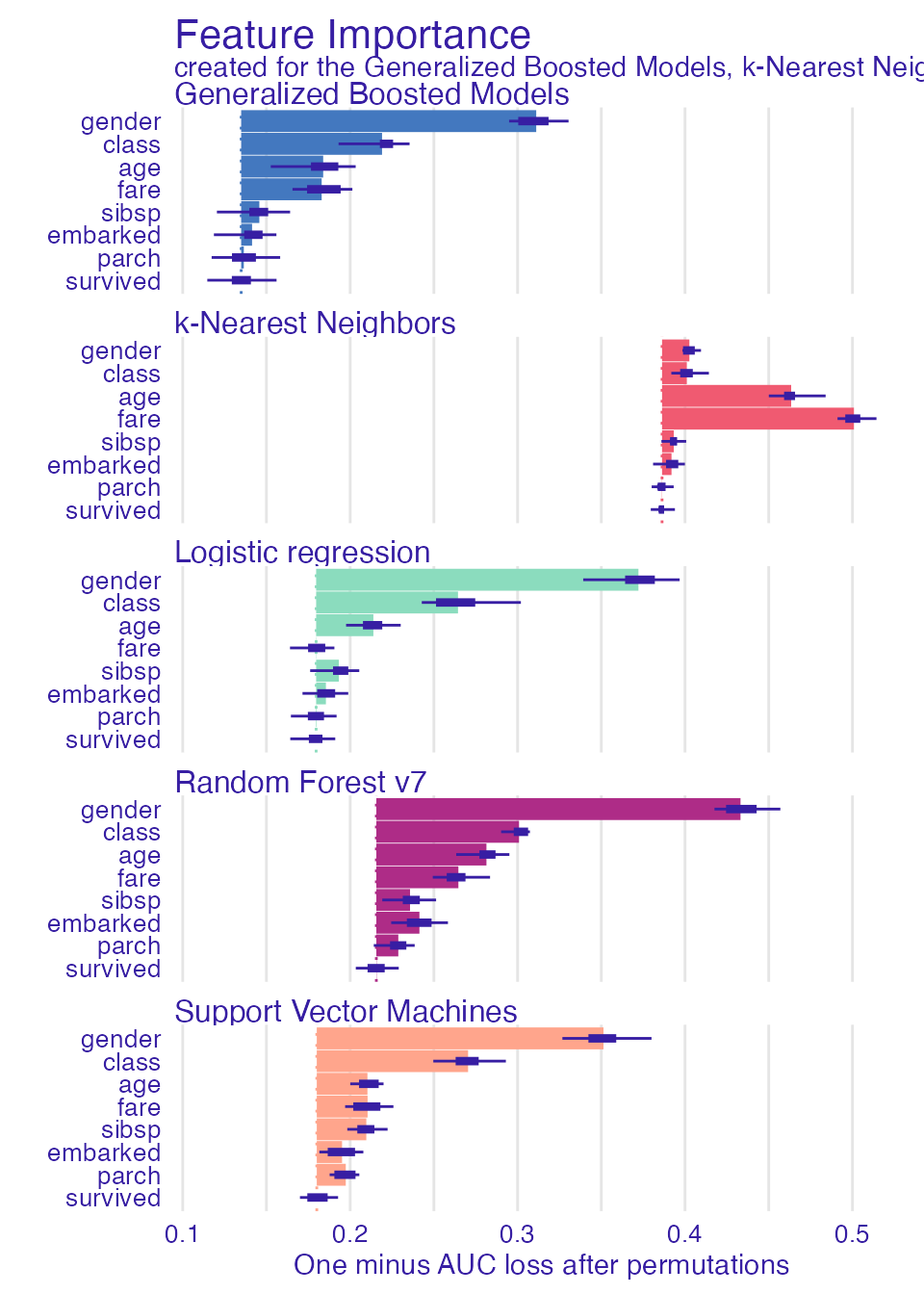

Single variable

vr_age_rf   <- model_profile(explain_titanic_rf, variables = "age")
vr_age_lmr  <- model_profile(explain_titanic_lmr, variables = "age")
vr_age_gbm  <- model_profile(explain_titanic_gbm, variables = "age")
vr_age_svm  <- model_profile(explain_titanic_svm, variables = "age")
vr_age_knn  <- model_profile(explain_titanic_knn, variables = "age")
plot(vr_age_rf$agr_profiles, 
     vr_age_lmr$agr_profiles, 
     vr_age_gbm$agr_profiles, 
     vr_age_svm$agr_profiles, 
     vr_age_knn$agr_profiles)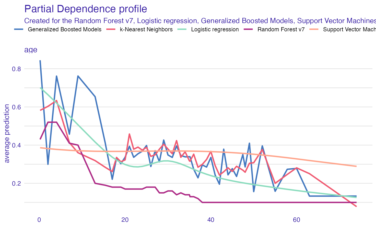

Instance level explanations

sp_rf <- predict_parts(explain_titanic_rf, new_passanger)
plot(sp_rf)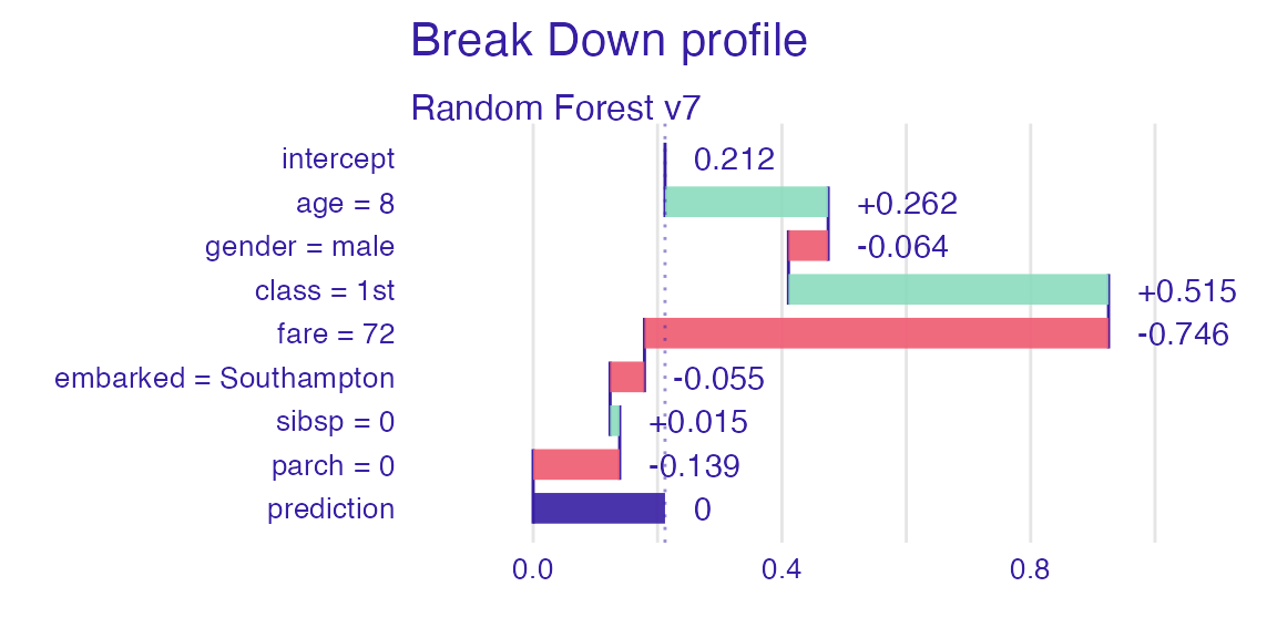

sp_lmr <- predict_parts(explain_titanic_lmr, new_passanger)
plot(sp_lmr)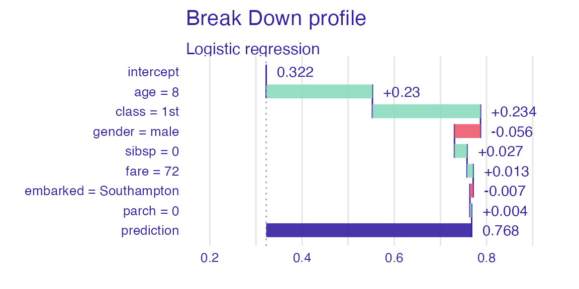

sp_gbm <- predict_parts(explain_titanic_gbm, new_passanger)
plot(sp_gbm)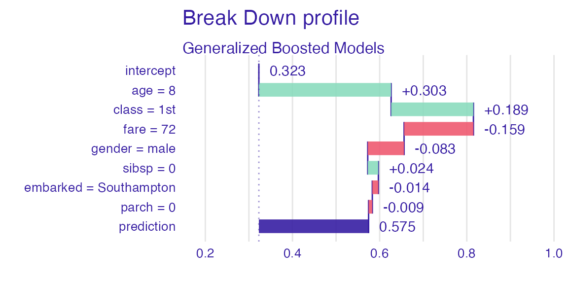

sp_svm <- predict_parts(explain_titanic_svm, new_passanger)
plot(sp_svm)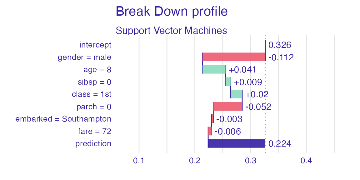

sp_knn <- predict_parts(explain_titanic_knn, new_passanger)
plot(sp_knn)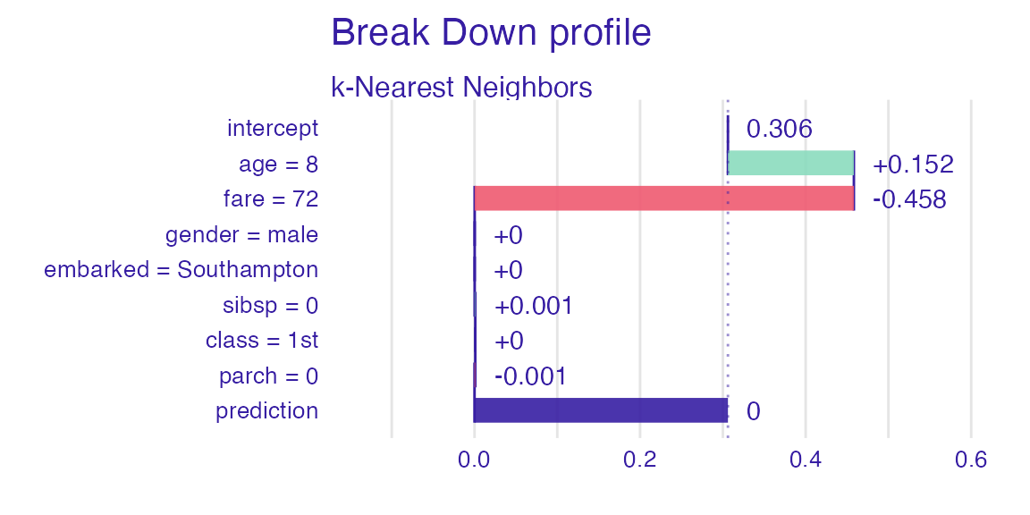

Session info

sessionInfo()

#> R version 4.2.3 (2023-03-15)
#> Platform: x86_64-apple-darwin17.0 (64-bit)
#> Running under: macOS Big Sur ... 10.16
#> 
#> Matrix products: default
#> BLAS:   /Library/Frameworks/R.framework/Versions/4.2/Resources/lib/libRblas.0.dylib
#> LAPACK: /Library/Frameworks/R.framework/Versions/4.2/Resources/lib/libRlapack.dylib
#> 
#> locale:
#> [1] en_US.UTF-8/en_US.UTF-8/en_US.UTF-8/C/en_US.UTF-8/en_US.UTF-8
#> 
#> attached base packages:
#> [1] stats     graphics  grDevices utils     datasets  methods   base     
#> 
#> other attached packages:
#>  [1] caret_6.0-94    e1071_1.7-13    gbm_2.1.8.1     rms_6.5-0      
#>  [5] SparseM_1.81    ggplot2_3.4.1   lattice_0.20-45 survival_3.5-3 
#>  [9] Hmisc_5.0-1     ranger_0.14.1   DALEX_2.5.1    
#> 
#> loaded via a namespace (and not attached):
#>   [1] nlme_3.1-162         fs_1.6.1             lubridate_1.9.2     
#>   [4] rprojroot_2.0.3      tools_4.2.3          backports_1.4.1     
#>   [7] bslib_0.4.2          utf8_1.2.3           R6_2.5.1            
#>  [10] rpart_4.1.19         colorspace_2.1-0     nnet_7.3-18         
#>  [13] withr_2.5.0          tidyselect_1.2.0     gridExtra_2.3       
#>  [16] compiler_4.2.3       textshaping_0.3.6    cli_3.6.0           
#>  [19] quantreg_5.94        htmlTable_2.4.1      desc_1.4.2          
#>  [22] sandwich_3.0-2       labeling_0.4.2       sass_0.4.5          
#>  [25] scales_1.2.1         checkmate_2.1.0      polspline_1.1.22    
#>  [28] mvtnorm_1.1-3        proxy_0.4-27         pkgdown_2.0.7       
#>  [31] systemfonts_1.0.4    stringr_1.5.0        digest_0.6.31       
#>  [34] foreign_0.8-84       ingredients_2.3.0    rmarkdown_2.20      
#>  [37] iBreakDown_2.0.1     base64enc_0.1-3      pkgconfig_2.0.3     
#>  [40] htmltools_0.5.4      parallelly_1.34.0    fastmap_1.1.1       
#>  [43] highr_0.10           htmlwidgets_1.6.2    rlang_1.1.0         
#>  [46] rstudioapi_0.14      jquerylib_0.1.4      farver_2.1.1        
#>  [49] generics_0.1.3       zoo_1.8-11           jsonlite_1.8.4      
#>  [52] ModelMetrics_1.2.2.2 dplyr_1.1.1          magrittr_2.0.3      
#>  [55] Formula_1.2-5        Matrix_1.5-3         Rcpp_1.0.10         
#>  [58] munsell_0.5.0        fansi_1.0.4          lifecycle_1.0.3     
#>  [61] pROC_1.18.0          stringi_1.7.12       multcomp_1.4-23     
#>  [64] yaml_2.3.7           MASS_7.3-58.2        plyr_1.8.8          
#>  [67] recipes_1.0.5        grid_4.2.3           parallel_4.2.3      
#>  [70] listenv_0.9.0        splines_4.2.3        knitr_1.42          
#>  [73] pillar_1.9.0         stats4_4.2.3         reshape2_1.4.4      
#>  [76] future.apply_1.10.0  codetools_0.2-19     glue_1.6.2          
#>  [79] evaluate_0.20        data.table_1.14.8    vctrs_0.6.1         
#>  [82] foreach_1.5.2        MatrixModels_0.5-1   gtable_0.3.3        
#>  [85] purrr_1.0.1          future_1.32.0        cachem_1.0.7        
#>  [88] gower_1.0.1          xfun_0.37            prodlim_2019.11.13  
#>  [91] ragg_1.2.5           class_7.3-21         timeDate_4022.108   
#>  [94] tibble_3.2.1         iterators_1.0.14     hardhat_1.2.0       
#>  [97] memoise_2.0.1        lava_1.7.2.1         cluster_2.1.4       
#> [100] timechange_0.2.0     globals_0.16.2       TH.data_1.1-1       
#> [103] ipred_0.9-14

Przemyslaw Biecek

2023-03-22

Data for Titanic survival

Model for Titanic survival

Explainer for Titanic survival

Variable importance plots

Variable effects

Age

Passenger class

Fare

Embarked

Instance level explanations

More models

Logistic regression

Generalized Boosted Models (GBM)

Support Vector Machines (SVM)

k-Nearest Neighbors (kNN)

Variable performance

Single variable

Instance level explanations

Session info