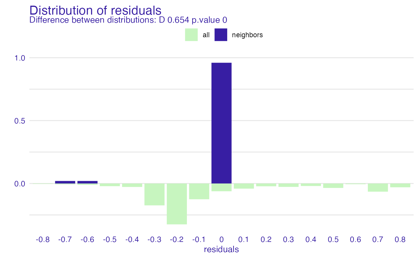
This function performs local diagnostic of residuals. For a single instance its neighbors are identified in the validation data. Residuals are calculated for neighbors and plotted against residuals for all data. Find information how to use this function here: https://ema.drwhy.ai/localDiagnostics.html.
predict_diagnostics(
  explainer,
  new_observation,
  variables = NULL,
  ...,
  nbins = 20,
  neighbors = 50,
  distance = gower::gower_dist
)

individual_diagnostics(
  explainer,
  new_observation,
  variables = NULL,
  ...,
  nbins = 20,
  neighbors = 50,
  distance = gower::gower_dist
)
Arguments
- explainer
a model to be explained, preprocessed by the 'explain' function
- new_observation
a new observation for which predictions need to be explained
- variables
character - name of variables to be explained
- ...
other parameters
- nbins
number of bins for the histogram. By default 20
- neighbors
number of neighbors for histogram. By default 50.
- distance
the distance function, by default the
gower_dist()function.
Value
An object of the class 'predict_diagnostics'. It's a data frame with calculated distribution of residuals.
References
Explanatory Model Analysis. Explore, Explain, and Examine Predictive Models. https://ema.drwhy.ai/
Examples
# \donttest{
library("ranger")
titanic_glm_model <- ranger(survived ~ gender + age + class + fare + sibsp + parch,
data = titanic_imputed)
explainer_glm <- explain(titanic_glm_model,
data = titanic_imputed,
y = titanic_imputed$survived)
#> Preparation of a new explainer is initiated
#> -> model label : ranger ( default )
#> -> data : 2207 rows 8 cols
#> -> target variable : 2207 values
#> -> predict function : yhat.ranger will be used ( default )
#> -> predicted values : No value for predict function target column. ( default )
#> -> model_info : package ranger , ver. 0.14.1 , task regression ( default )
#> -> predicted values : numerical, min = 0.008737237 , mean = 0.3217409 , max = 0.9959586
#> -> residual function : difference between y and yhat ( default )
#> -> residuals : numerical, min = -0.7807803 , mean = 0.0004158392 , max = 0.8781949
#> A new explainer has been created!
johny_d <- titanic_imputed[24, c("gender", "age", "class", "fare", "sibsp", "parch")]
id_johny <- predict_diagnostics(explainer_glm, johny_d, variables = NULL)
#> Warning: p-value will be approximate in the presence of ties
id_johny
#>
#> Asymptotic two-sample Kolmogorov-Smirnov test
#>
#> data: residuals_other and residuals_sel
#> D = 0.65356, p-value < 2.2e-16
#> alternative hypothesis: two-sided
#>
plot(id_johny)
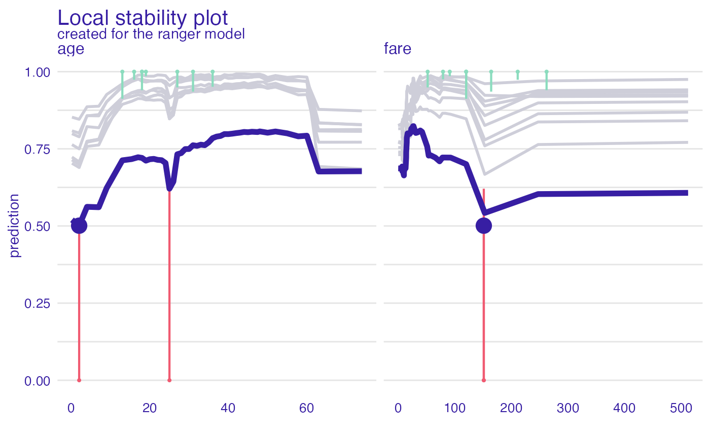
 id_johny <- predict_diagnostics(explainer_glm, johny_d,
neighbors = 10,
variables = c("age", "fare"))
id_johny
#> Top profiles :
#> gender age class fare sibsp parch _yhat_ _vname_ _ids_ _label_
#> 24 female 0.1666667 1st 151.16 1 2 0.5200738 age 24 ranger
#> 24.1 female 2.0000000 1st 151.16 1 2 0.5009633 age 24 ranger
#> 24.2 female 4.0000000 1st 151.16 1 2 0.5620734 age 24 ranger
#> 24.3 female 7.0000000 1st 151.16 1 2 0.5608068 age 24 ranger
#> 24.4 female 9.0000000 1st 151.16 1 2 0.6228031 age 24 ranger
#> 24.5 female 13.0000000 1st 151.16 1 2 0.7127380 age 24 ranger
#>
#>
#> Top observations:
#> gender age class fare sibsp parch _yhat_ _label_ _ids_
#> 24 female 2 1st 151.16 1 2 0.5009633 ranger 1
plot(id_johny)
id_johny <- predict_diagnostics(explainer_glm, johny_d,
neighbors = 10,
variables = c("age", "fare"))
id_johny
#> Top profiles :
#> gender age class fare sibsp parch _yhat_ _vname_ _ids_ _label_
#> 24 female 0.1666667 1st 151.16 1 2 0.5200738 age 24 ranger
#> 24.1 female 2.0000000 1st 151.16 1 2 0.5009633 age 24 ranger
#> 24.2 female 4.0000000 1st 151.16 1 2 0.5620734 age 24 ranger
#> 24.3 female 7.0000000 1st 151.16 1 2 0.5608068 age 24 ranger
#> 24.4 female 9.0000000 1st 151.16 1 2 0.6228031 age 24 ranger
#> 24.5 female 13.0000000 1st 151.16 1 2 0.7127380 age 24 ranger
#>
#>
#> Top observations:
#> gender age class fare sibsp parch _yhat_ _label_ _ids_
#> 24 female 2 1st 151.16 1 2 0.5009633 ranger 1
plot(id_johny)
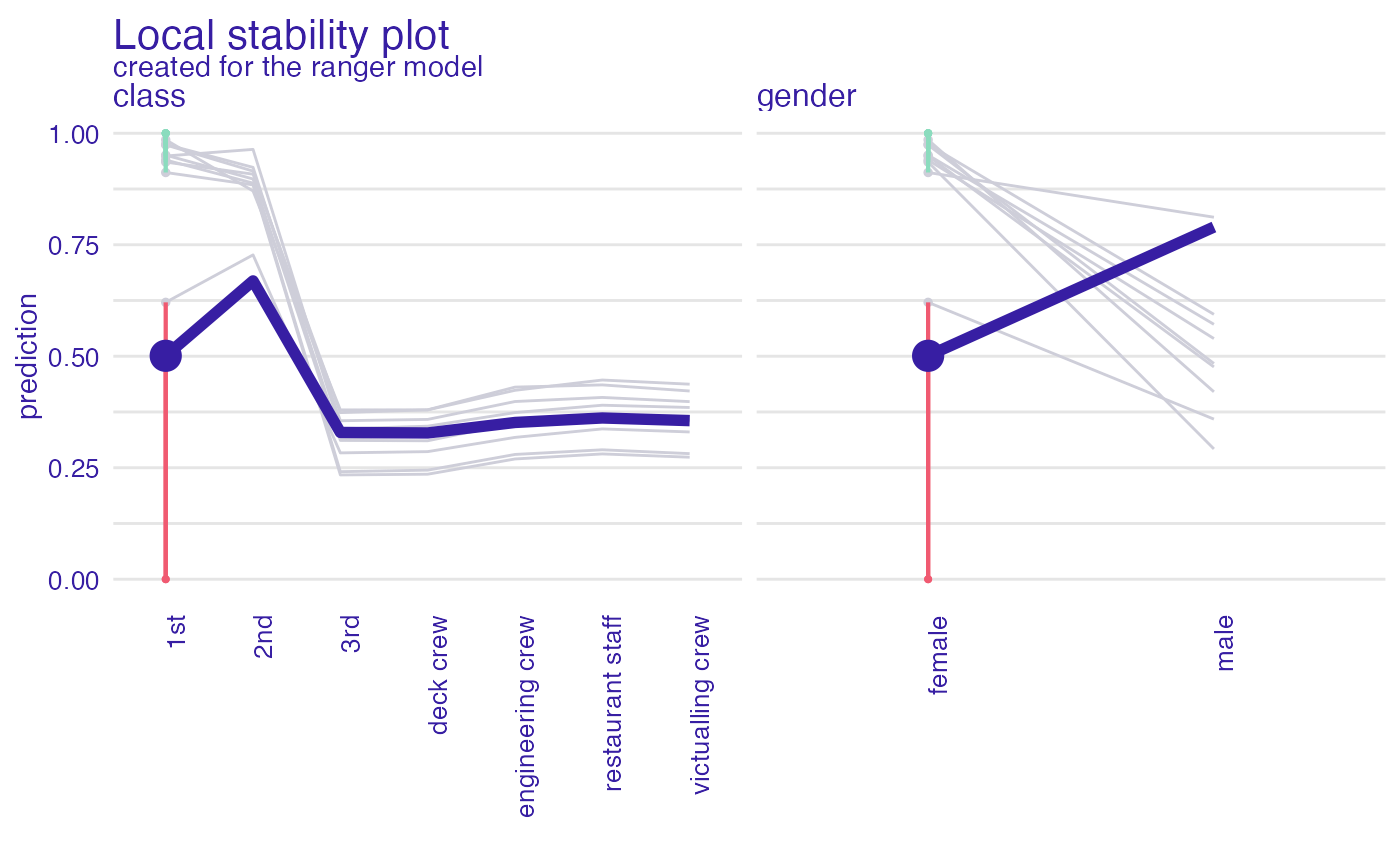
 id_johny <- predict_diagnostics(explainer_glm,
johny_d,
neighbors = 10,
variables = c("class", "gender"))
id_johny
#> Top profiles :
#> gender age class fare sibsp parch _yhat_ _vname_ _ids_
#> 24 female 2 1st 151.16 1 2 0.5009633 class 24
#> 24.1 female 2 2nd 151.16 1 2 0.6689694 class 24
#> 24.2 female 2 3rd 151.16 1 2 0.3290978 class 24
#> 24.3 female 2 deck crew 151.16 1 2 0.3279391 class 24
#> 24.4 female 2 engineering crew 151.16 1 2 0.3514825 class 24
#> 24.5 female 2 restaurant staff 151.16 1 2 0.3615452 class 24
#> _label_
#> 24 ranger
#> 24.1 ranger
#> 24.2 ranger
#> 24.3 ranger
#> 24.4 ranger
#> 24.5 ranger
#>
#>
#> Top observations:
#> gender age class fare sibsp parch _yhat_ _label_ _ids_
#> 24 female 2 1st 151.16 1 2 0.5009633 ranger 1
plot(id_johny)
#> 'variable_type' changed to 'categorical' due to lack of numerical variables.
#> 'variable_type' changed to 'categorical' due to lack of numerical variables.
id_johny <- predict_diagnostics(explainer_glm,
johny_d,
neighbors = 10,
variables = c("class", "gender"))
id_johny
#> Top profiles :
#> gender age class fare sibsp parch _yhat_ _vname_ _ids_
#> 24 female 2 1st 151.16 1 2 0.5009633 class 24
#> 24.1 female 2 2nd 151.16 1 2 0.6689694 class 24
#> 24.2 female 2 3rd 151.16 1 2 0.3290978 class 24
#> 24.3 female 2 deck crew 151.16 1 2 0.3279391 class 24
#> 24.4 female 2 engineering crew 151.16 1 2 0.3514825 class 24
#> 24.5 female 2 restaurant staff 151.16 1 2 0.3615452 class 24
#> _label_
#> 24 ranger
#> 24.1 ranger
#> 24.2 ranger
#> 24.3 ranger
#> 24.4 ranger
#> 24.5 ranger
#>
#>
#> Top observations:
#> gender age class fare sibsp parch _yhat_ _label_ _ids_
#> 24 female 2 1st 151.16 1 2 0.5009633 ranger 1
plot(id_johny)
#> 'variable_type' changed to 'categorical' due to lack of numerical variables.
#> 'variable_type' changed to 'categorical' due to lack of numerical variables.
 # }
# }