Plots Aggregated Profiles
Source:R/plot_aggregated_profiles.R
plot.aggregated_profiles_explainer.RdFunction plot.aggregated_profiles_explainer plots partial dependence plot or accumulated effect plot.
It works in a similar way to plot.ceteris_paribus, but instead of individual profiles
show average profiles for each variable listed in the variables vector.
# S3 method for aggregated_profiles_explainer
plot(
  x,
  ...,
  size = 1,
  alpha = 1,
  color = "_label_",
  facet_ncol = NULL,
  facet_scales = "free_x",
  variables = NULL,
  title = NULL,
  subtitle = NULL
)
Arguments
- x
a ceteris paribus explainer produced with function
aggregate_profiles()- ...
other explainers that shall be plotted together
- size
a numeric. Size of lines to be plotted
- alpha
a numeric between
0and1. Opacity of lines- color
a character. Either name of a color, or hex code for a color, or
_label_if models shall be colored, or_ids_if instances shall be colored- facet_ncol
number of columns for the
facet_wrap- facet_scales
a character value for the
facet_wrap. Default is"free_x".- variables
if not
NULLthen onlyvariableswill be presented- title
a character. Partial and accumulated dependence explainers have deafult value.
- subtitle
a character. If
NULLvalue will be dependent on model usage.
Value
a ggplot2 object
References
Explanatory Model Analysis. Explore, Explain, and Examine Predictive Models. https://ema.drwhy.ai/
Examples
library("DALEX")
library("ingredients")
model_titanic_glm <- glm(survived ~ gender + age + fare,
data = titanic_imputed, family = "binomial")
explain_titanic_glm <- explain(model_titanic_glm,
data = titanic_imputed[,-8],
y = titanic_imputed[,8],
verbose = FALSE)
pdp_rf_p <- partial_dependence(explain_titanic_glm, N = 50)
pdp_rf_p$`_label_` <- "RF_partial"
pdp_rf_l <- conditional_dependence(explain_titanic_glm, N = 50)
pdp_rf_l$`_label_` <- "RF_local"
pdp_rf_a<- accumulated_dependence(explain_titanic_glm, N = 50)
pdp_rf_a$`_label_` <- "RF_accumulated"
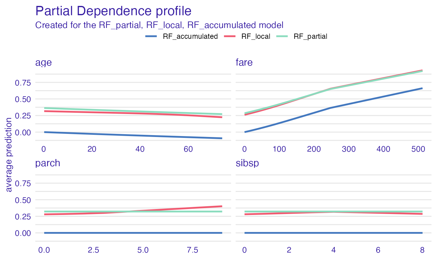
head(pdp_rf_p)
#> Top profiles :
#> _vname_ _label_ _x_ _yhat_ _ids_
#> 1 fare RF_partial 0.0000000 0.2848672 0
#> 2 parch RF_partial 0.0000000 0.3221967 0
#> 3 sibsp RF_partial 0.0000000 0.3221967 0
#> 4 age RF_partial 0.1666667 0.3632136 0
#> 5 parch RF_partial 1.0000000 0.3221967 0
#> 6 sibsp RF_partial 1.0000000 0.3221967 0
plot(pdp_rf_p, pdp_rf_l, pdp_rf_a, color = "_label_")
 # \donttest{
library("ranger")
model_titanic_rf <- ranger(survived ~., data = titanic_imputed, probability = TRUE)
explain_titanic_rf <- explain(model_titanic_rf,
data = titanic_imputed[,-8],
y = titanic_imputed[,8],
label = "ranger forest",
verbose = FALSE)
selected_passangers <- select_sample(titanic_imputed, n = 100)
cp_rf <- ceteris_paribus(explain_titanic_rf, selected_passangers)
cp_rf
#> Top profiles :
#> gender age class embarked fare sibsp parch _yhat_
#> 515 female 45 2nd Southampton 10.1000 0 0 0.8193970
#> 515.1 male 45 2nd Southampton 10.1000 0 0 0.1225410
#> 604 female 17 3rd Southampton 7.1701 1 0 0.4562376
#> 604.1 male 17 3rd Southampton 7.1701 1 0 0.1100723
#> 1430 female 25 engineering crew Southampton 0.0000 0 0 0.7582714
#> 1430.1 male 25 engineering crew Southampton 0.0000 0 0 0.2340968
#> _vname_ _ids_ _label_
#> 515 gender 515 ranger forest
#> 515.1 gender 515 ranger forest
#> 604 gender 604 ranger forest
#> 604.1 gender 604 ranger forest
#> 1430 gender 1430 ranger forest
#> 1430.1 gender 1430 ranger forest
#>
#>
#> Top observations:
#> gender age class embarked fare sibsp parch _yhat_
#> 515 male 45 2nd Southampton 10.1000 0 0 0.1225410
#> 604 male 17 3rd Southampton 7.1701 1 0 0.1100723
#> 1430 male 25 engineering crew Southampton 0.0000 0 0 0.2340968
#> 865 male 20 3rd Cherbourg 7.0406 0 0 0.1103113
#> 452 female 17 3rd Queenstown 7.1408 0 0 0.6707266
#> 1534 male 38 victualling crew Southampton 0.0000 0 0 0.1745903
#> _label_ _ids_
#> 515 ranger forest 1
#> 604 ranger forest 2
#> 1430 ranger forest 3
#> 865 ranger forest 4
#> 452 ranger forest 5
#> 1534 ranger forest 6
pdp_rf_p <- aggregate_profiles(cp_rf, variables = "age", type = "partial")
pdp_rf_p$`_label_` <- "RF_partial"
pdp_rf_c <- aggregate_profiles(cp_rf, variables = "age", type = "conditional")
pdp_rf_c$`_label_` <- "RF_conditional"
pdp_rf_a <- aggregate_profiles(cp_rf, variables = "age", type = "accumulated")
pdp_rf_a$`_label_` <- "RF_accumulated"
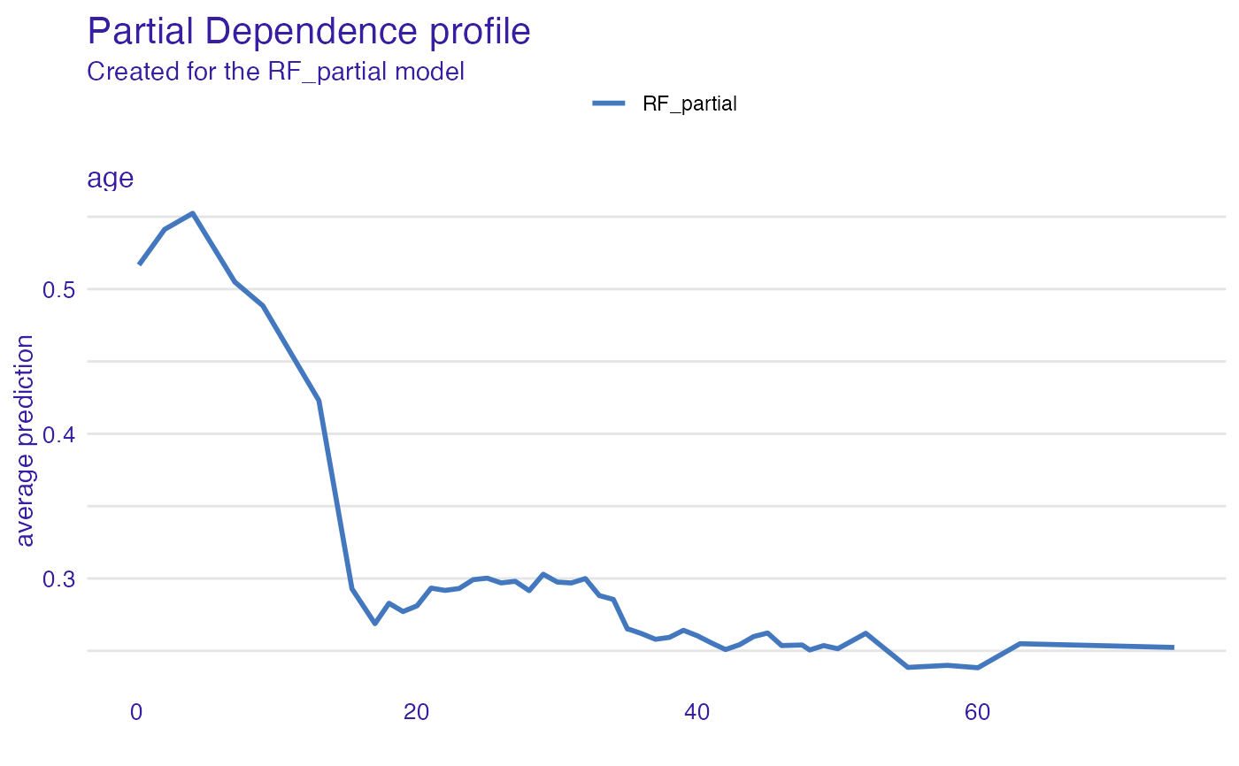
head(pdp_rf_p)
#> Top profiles :
#> _vname_ _label_ _x_ _yhat_ _ids_
#> 1 age RF_partial 0.1666667 0.5167099 0
#> 2 age RF_partial 2.0000000 0.5412926 0
#> 3 age RF_partial 4.0000000 0.5523954 0
#> 4 age RF_partial 7.0000000 0.5049700 0
#> 5 age RF_partial 9.0000000 0.4885480 0
#> 6 age RF_partial 13.0000000 0.4229736 0
plot(pdp_rf_p)
# \donttest{
library("ranger")
model_titanic_rf <- ranger(survived ~., data = titanic_imputed, probability = TRUE)
explain_titanic_rf <- explain(model_titanic_rf,
data = titanic_imputed[,-8],
y = titanic_imputed[,8],
label = "ranger forest",
verbose = FALSE)
selected_passangers <- select_sample(titanic_imputed, n = 100)
cp_rf <- ceteris_paribus(explain_titanic_rf, selected_passangers)
cp_rf
#> Top profiles :
#> gender age class embarked fare sibsp parch _yhat_
#> 515 female 45 2nd Southampton 10.1000 0 0 0.8193970
#> 515.1 male 45 2nd Southampton 10.1000 0 0 0.1225410
#> 604 female 17 3rd Southampton 7.1701 1 0 0.4562376
#> 604.1 male 17 3rd Southampton 7.1701 1 0 0.1100723
#> 1430 female 25 engineering crew Southampton 0.0000 0 0 0.7582714
#> 1430.1 male 25 engineering crew Southampton 0.0000 0 0 0.2340968
#> _vname_ _ids_ _label_
#> 515 gender 515 ranger forest
#> 515.1 gender 515 ranger forest
#> 604 gender 604 ranger forest
#> 604.1 gender 604 ranger forest
#> 1430 gender 1430 ranger forest
#> 1430.1 gender 1430 ranger forest
#>
#>
#> Top observations:
#> gender age class embarked fare sibsp parch _yhat_
#> 515 male 45 2nd Southampton 10.1000 0 0 0.1225410
#> 604 male 17 3rd Southampton 7.1701 1 0 0.1100723
#> 1430 male 25 engineering crew Southampton 0.0000 0 0 0.2340968
#> 865 male 20 3rd Cherbourg 7.0406 0 0 0.1103113
#> 452 female 17 3rd Queenstown 7.1408 0 0 0.6707266
#> 1534 male 38 victualling crew Southampton 0.0000 0 0 0.1745903
#> _label_ _ids_
#> 515 ranger forest 1
#> 604 ranger forest 2
#> 1430 ranger forest 3
#> 865 ranger forest 4
#> 452 ranger forest 5
#> 1534 ranger forest 6
pdp_rf_p <- aggregate_profiles(cp_rf, variables = "age", type = "partial")
pdp_rf_p$`_label_` <- "RF_partial"
pdp_rf_c <- aggregate_profiles(cp_rf, variables = "age", type = "conditional")
pdp_rf_c$`_label_` <- "RF_conditional"
pdp_rf_a <- aggregate_profiles(cp_rf, variables = "age", type = "accumulated")
pdp_rf_a$`_label_` <- "RF_accumulated"
head(pdp_rf_p)
#> Top profiles :
#> _vname_ _label_ _x_ _yhat_ _ids_
#> 1 age RF_partial 0.1666667 0.5167099 0
#> 2 age RF_partial 2.0000000 0.5412926 0
#> 3 age RF_partial 4.0000000 0.5523954 0
#> 4 age RF_partial 7.0000000 0.5049700 0
#> 5 age RF_partial 9.0000000 0.4885480 0
#> 6 age RF_partial 13.0000000 0.4229736 0
plot(pdp_rf_p)
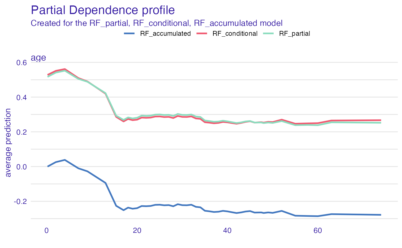
 plot(pdp_rf_p, pdp_rf_c, pdp_rf_a)
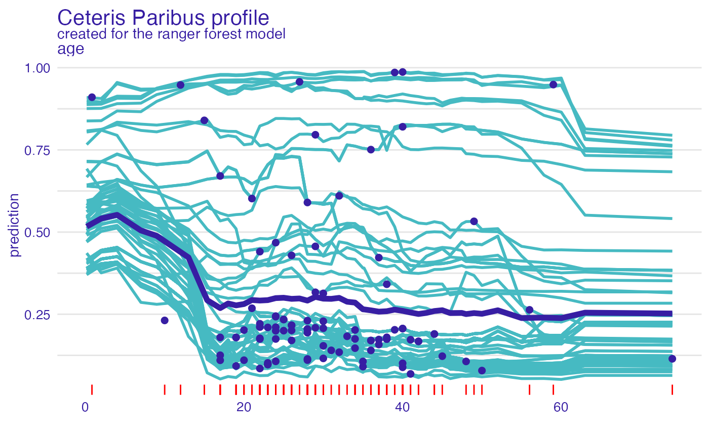
 plot(cp_rf, variables = "age") +
show_observations(cp_rf, variables = "age") +
show_rugs(cp_rf, variables = "age", color = "red") +
show_aggregated_profiles(pdp_rf_p, size = 2)
plot(cp_rf, variables = "age") +
show_observations(cp_rf, variables = "age") +
show_rugs(cp_rf, variables = "age", color = "red") +
show_aggregated_profiles(pdp_rf_p, size = 2)
 # }
# }