Adds a Layer with Rugs to a Profile Plot

Function show_rugs adds a layer to a plot created with plot.ceteris_paribus_explainer for selected observations. Various parameters help to decide what should be plotted, profiles, aggregated profiles, points or rugs.

show_rugs(
  x,
  ...,
  size = 0.5,
  alpha = 1,
  color = "#371ea3",
  variable_type = "numerical",
  sides = "b",
  variables = NULL
)

Arguments

x

a ceteris paribus explainer produced with function ceteris_paribus()

...

other explainers that shall be plotted together

size

a numeric. Size of lines to be plotted

alpha

a numeric between 0 and 1. Opacity of lines

color

a character. Either name of a color or name of a variable that should be used for coloring

variable_type

a character. If numerical then only numerical variables will be plotted. If categorical then only categorical variables will be plotted.

sides

a string containing any of "trbl", for top, right, bottom, and left. Passed to geom rug.

variables

if not NULL then only variables will be presented

Value

a ggplot2 layer

References

Explanatory Model Analysis. Explore, Explain, and Examine Predictive Models. https://ema.drwhy.ai/

Examples

library("DALEX")
library("ingredients")
titanic_small <- select_sample(titanic_imputed, n = 500, seed = 1313)

# build a model
model_titanic_glm <- glm(survived ~ gender + age + fare,
                         data = titanic_small,
                         family = "binomial")

explain_titanic_glm <- explain(model_titanic_glm,
                               data = titanic_small[,-8],
                               y = titanic_small[,8])
#> Preparation of a new explainer is initiated
#>   -> model label       :  lm  (  default  )
#>   -> data              :  500  rows  7  cols 
#>   -> target variable   :  500  values 
#>   -> predict function  :  yhat.glm  will be used (  default  )
#>   -> predicted values  :  No value for predict function target column. (  default  )
#>   -> model_info        :  package stats , ver. 4.2.2 , task classification (  default  ) 
#>   -> predicted values  :  numerical, min =  0.0795294 , mean =  0.302 , max =  0.9859411  
#>   -> residual function :  difference between y and yhat (  default  )
#>   -> residuals         :  numerical, min =  -0.8204691 , mean =  8.796651e-12 , max =  0.8567173  
#>   A new explainer has been created!  

cp_glm <- ceteris_paribus(explain_titanic_glm, titanic_small[1,])
cp_glm
#> Top profiles    : 
#>         gender   age class    embarked fare sibsp parch    _yhat_ _vname_ _ids_
#> 515     female 45.00   2nd Southampton 10.1     0     0 0.5595687  gender   515
#> 515.1     male 45.00   2nd Southampton 10.1     0     0 0.1448038  gender   515
#> 5151      male  0.75   2nd Southampton 10.1     0     0 0.3135247     age   515
#> 515.110   male  2.99   2nd Southampton 10.1     0     0 0.3028164     age   515
#> 515.2     male  4.98   2nd Southampton 10.1     0     0 0.2934793     age   515
#> 515.3     male  7.00   2nd Southampton 10.1     0     0 0.2841757     age   515
#>         _label_
#> 515          lm
#> 515.1        lm
#> 5151         lm
#> 515.110      lm
#> 515.2        lm
#> 515.3        lm
#> 
#> 
#> Top observations:
#>     gender age class    embarked fare sibsp parch    _yhat_ _label_ _ids_
#> 515   male  45   2nd Southampton 10.1     0     0 0.1448038      lm     1

# \donttest{
library("ranger")

rf_model <- ranger(survived ~., data = titanic_imputed, probability = TRUE)

explainer_rf <- explain(rf_model,
                        data = titanic_imputed[,-8],
                        y = titanic_imputed[,8],
                        label = "ranger forest",
                        verbose = FALSE)

selected_passangers <- select_sample(titanic_imputed, n = 100)
cp_rf <- ceteris_paribus(explainer_rf, selected_passangers)
cp_rf
#> Top profiles    : 
#>        gender age            class    embarked    fare sibsp parch    _yhat_
#> 515    female  45              2nd Southampton 10.1000     0     0 0.8130768
#> 515.1    male  45              2nd Southampton 10.1000     0     0 0.1134421
#> 604    female  17              3rd Southampton  7.1701     1     0 0.4691766
#> 604.1    male  17              3rd Southampton  7.1701     1     0 0.1146410
#> 1430   female  25 engineering crew Southampton  0.0000     0     0 0.7580796
#> 1430.1   male  25 engineering crew Southampton  0.0000     0     0 0.2382367
#>        _vname_ _ids_       _label_
#> 515     gender   515 ranger forest
#> 515.1   gender   515 ranger forest
#> 604     gender   604 ranger forest
#> 604.1   gender   604 ranger forest
#> 1430    gender  1430 ranger forest
#> 1430.1  gender  1430 ranger forest
#> 
#> 
#> Top observations:
#>      gender age            class    embarked    fare sibsp parch    _yhat_
#> 515    male  45              2nd Southampton 10.1000     0     0 0.1134421
#> 604    male  17              3rd Southampton  7.1701     1     0 0.1146410
#> 1430   male  25 engineering crew Southampton  0.0000     0     0 0.2382367
#> 865    male  20              3rd   Cherbourg  7.0406     0     0 0.1177139
#> 452  female  17              3rd  Queenstown  7.1408     0     0 0.6675361
#> 1534   male  38 victualling crew Southampton  0.0000     0     0 0.1723540
#>            _label_ _ids_
#> 515  ranger forest     1
#> 604  ranger forest     2
#> 1430 ranger forest     3
#> 865  ranger forest     4
#> 452  ranger forest     5
#> 1534 ranger forest     6

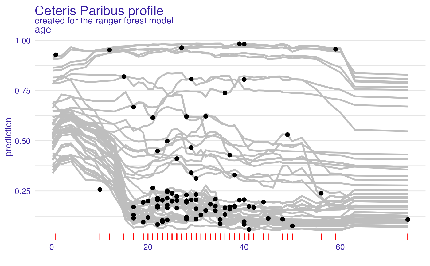
plot(cp_rf, variables = "age", color = "grey") +
show_observations(cp_rf, variables = "age", color = "black") +
  show_rugs(cp_rf, variables = "age", color = "red")

# }