Function plot.ceteris_paribus_explainer plots Individual Variable Profiles for selected observations.
Various parameters help to decide what should be plotted, profiles, aggregated profiles, points or rugs.
Find more details in Ceteris Paribus Chapter.
# S3 method for ceteris_paribus_explainer
plot(
  x,
  ...,
  size = 1,
  alpha = 1,
  color = "#46bac2",
  variable_type = "numerical",
  facet_ncol = NULL,
  facet_scales = NULL,
  variables = NULL,
  title = "Ceteris Paribus profile",
  subtitle = NULL,
  categorical_type = "profiles"
)
Arguments
- x
a ceteris paribus explainer produced with function
ceteris_paribus()- ...
other explainers that shall be plotted together
- size
a numeric. Size of lines to be plotted
- alpha
a numeric between
0and1. Opacity of lines- color
a character. Either name of a color or name of a variable that should be used for coloring
- variable_type
a character. If
numericalthen only numerical variables will be plotted. Ifcategoricalthen only categorical variables will be plotted.- facet_ncol
number of columns for the
facet_wrap- facet_scales
a character value for the
facet_wrap. Default is"free_x", but"free_y"ifcategorical_type="bars".- variables
if not
NULLthen onlyvariableswill be presented- title
a character. Plot title. By default "Ceteris Paribus profile".
- subtitle
a character. Plot subtitle. By default
NULL- then subtitle is set to "created for the XXX, YYY model", where XXX, YYY are labels of given explainers.- categorical_type
a character. How categorical variables shall be plotted? Either
"profiles"(default) or"bars"or"lines".
Value
a ggplot2 object
References
Explanatory Model Analysis. Explore, Explain, and Examine Predictive Models. https://ema.drwhy.ai/
Examples
library("DALEX")
model_titanic_glm <- glm(survived ~ gender + age + fare,
data = titanic_imputed, family = "binomial")
explain_titanic_glm <- explain(model_titanic_glm,
data = titanic_imputed[,-8],
y = titanic_imputed[,8],
verbose = FALSE)
cp_glm <- ceteris_paribus(explain_titanic_glm, titanic_imputed[1,])
cp_glm
#> Top profiles :
#> gender age class embarked fare sibsp parch _yhat_ _vname_
#> 1 female 42.0000000 3rd Southampton 7.11 0 0 0.6667679 gender
#> 1.1 male 42.0000000 3rd Southampton 7.11 0 0 0.1827040 gender
#> 11 male 0.1666667 3rd Southampton 7.11 0 0 0.2352754 age
#> 1.110 male 2.0000000 3rd Southampton 7.11 0 0 0.2327665 age
#> 1.2 male 4.0000000 3rd Southampton 7.11 0 0 0.2300508 age
#> 1.3 male 7.0000000 3rd Southampton 7.11 0 0 0.2260191 age
#> _ids_ _label_
#> 1 1 lm
#> 1.1 1 lm
#> 11 1 lm
#> 1.110 1 lm
#> 1.2 1 lm
#> 1.3 1 lm
#>
#>
#> Top observations:
#> gender age class embarked fare sibsp parch _yhat_ _label_ _ids_
#> 1 male 42 3rd Southampton 7.11 0 0 0.182704 lm 1
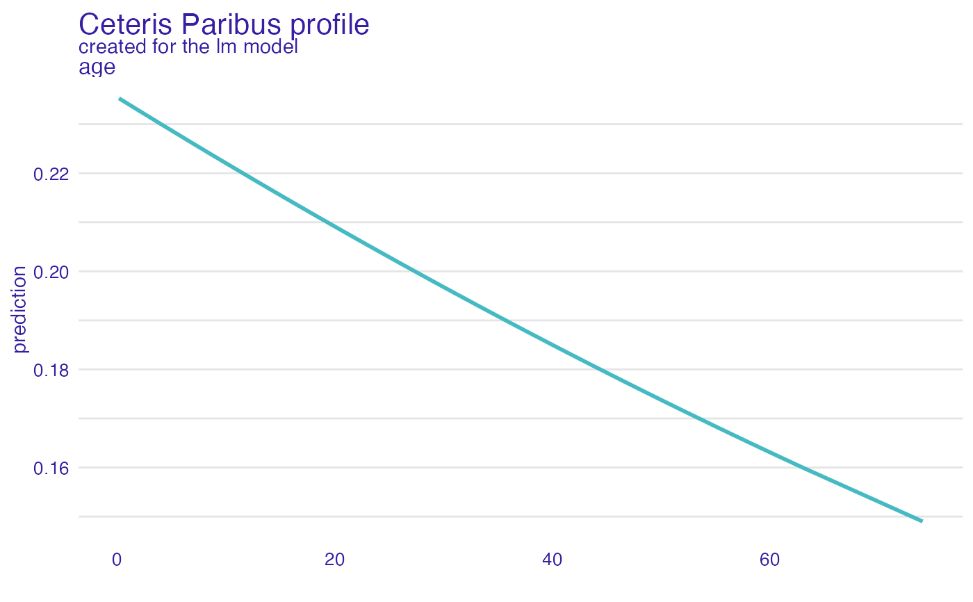
plot(cp_glm, variables = "age")
 # \donttest{
library("ranger")
model_titanic_rf <- ranger(survived ~., data = titanic_imputed, probability = TRUE)
explain_titanic_rf <- explain(model_titanic_rf,
data = titanic_imputed[,-8],
y = titanic_imputed[,8],
label = "ranger forest",
verbose = FALSE)
selected_passangers <- select_sample(titanic_imputed, n = 100)
cp_rf <- ceteris_paribus(explain_titanic_rf, selected_passangers)
cp_rf
#> Top profiles :
#> gender age class embarked fare sibsp parch _yhat_
#> 515 female 45 2nd Southampton 10.1000 0 0 0.7957940
#> 515.1 male 45 2nd Southampton 10.1000 0 0 0.1150837
#> 604 female 17 3rd Southampton 7.1701 1 0 0.4422906
#> 604.1 male 17 3rd Southampton 7.1701 1 0 0.1153614
#> 1430 female 25 engineering crew Southampton 0.0000 0 0 0.7682655
#> 1430.1 male 25 engineering crew Southampton 0.0000 0 0 0.2385723
#> _vname_ _ids_ _label_
#> 515 gender 515 ranger forest
#> 515.1 gender 515 ranger forest
#> 604 gender 604 ranger forest
#> 604.1 gender 604 ranger forest
#> 1430 gender 1430 ranger forest
#> 1430.1 gender 1430 ranger forest
#>
#>
#> Top observations:
#> gender age class embarked fare sibsp parch _yhat_
#> 515 male 45 2nd Southampton 10.1000 0 0 0.1150837
#> 604 male 17 3rd Southampton 7.1701 1 0 0.1153614
#> 1430 male 25 engineering crew Southampton 0.0000 0 0 0.2385723
#> 865 male 20 3rd Cherbourg 7.0406 0 0 0.1160834
#> 452 female 17 3rd Queenstown 7.1408 0 0 0.6609725
#> 1534 male 38 victualling crew Southampton 0.0000 0 0 0.1725586
#> _label_ _ids_
#> 515 ranger forest 1
#> 604 ranger forest 2
#> 1430 ranger forest 3
#> 865 ranger forest 4
#> 452 ranger forest 5
#> 1534 ranger forest 6
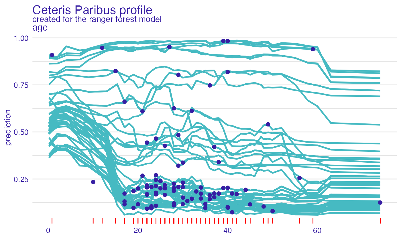
plot(cp_rf, variables = "age") +
show_observations(cp_rf, variables = "age") +
show_rugs(cp_rf, variables = "age", color = "red")
# \donttest{
library("ranger")
model_titanic_rf <- ranger(survived ~., data = titanic_imputed, probability = TRUE)
explain_titanic_rf <- explain(model_titanic_rf,
data = titanic_imputed[,-8],
y = titanic_imputed[,8],
label = "ranger forest",
verbose = FALSE)
selected_passangers <- select_sample(titanic_imputed, n = 100)
cp_rf <- ceteris_paribus(explain_titanic_rf, selected_passangers)
cp_rf
#> Top profiles :
#> gender age class embarked fare sibsp parch _yhat_
#> 515 female 45 2nd Southampton 10.1000 0 0 0.7957940
#> 515.1 male 45 2nd Southampton 10.1000 0 0 0.1150837
#> 604 female 17 3rd Southampton 7.1701 1 0 0.4422906
#> 604.1 male 17 3rd Southampton 7.1701 1 0 0.1153614
#> 1430 female 25 engineering crew Southampton 0.0000 0 0 0.7682655
#> 1430.1 male 25 engineering crew Southampton 0.0000 0 0 0.2385723
#> _vname_ _ids_ _label_
#> 515 gender 515 ranger forest
#> 515.1 gender 515 ranger forest
#> 604 gender 604 ranger forest
#> 604.1 gender 604 ranger forest
#> 1430 gender 1430 ranger forest
#> 1430.1 gender 1430 ranger forest
#>
#>
#> Top observations:
#> gender age class embarked fare sibsp parch _yhat_
#> 515 male 45 2nd Southampton 10.1000 0 0 0.1150837
#> 604 male 17 3rd Southampton 7.1701 1 0 0.1153614
#> 1430 male 25 engineering crew Southampton 0.0000 0 0 0.2385723
#> 865 male 20 3rd Cherbourg 7.0406 0 0 0.1160834
#> 452 female 17 3rd Queenstown 7.1408 0 0 0.6609725
#> 1534 male 38 victualling crew Southampton 0.0000 0 0 0.1725586
#> _label_ _ids_
#> 515 ranger forest 1
#> 604 ranger forest 2
#> 1430 ranger forest 3
#> 865 ranger forest 4
#> 452 ranger forest 5
#> 1534 ranger forest 6
plot(cp_rf, variables = "age") +
show_observations(cp_rf, variables = "age") +
show_rugs(cp_rf, variables = "age", color = "red")
 selected_passangers <- select_sample(titanic_imputed, n = 1)
selected_passangers
#> gender age class embarked fare sibsp parch survived
#> 515 male 45 2nd Southampton 10.1 0 0 0
cp_rf <- ceteris_paribus(explain_titanic_rf, selected_passangers)
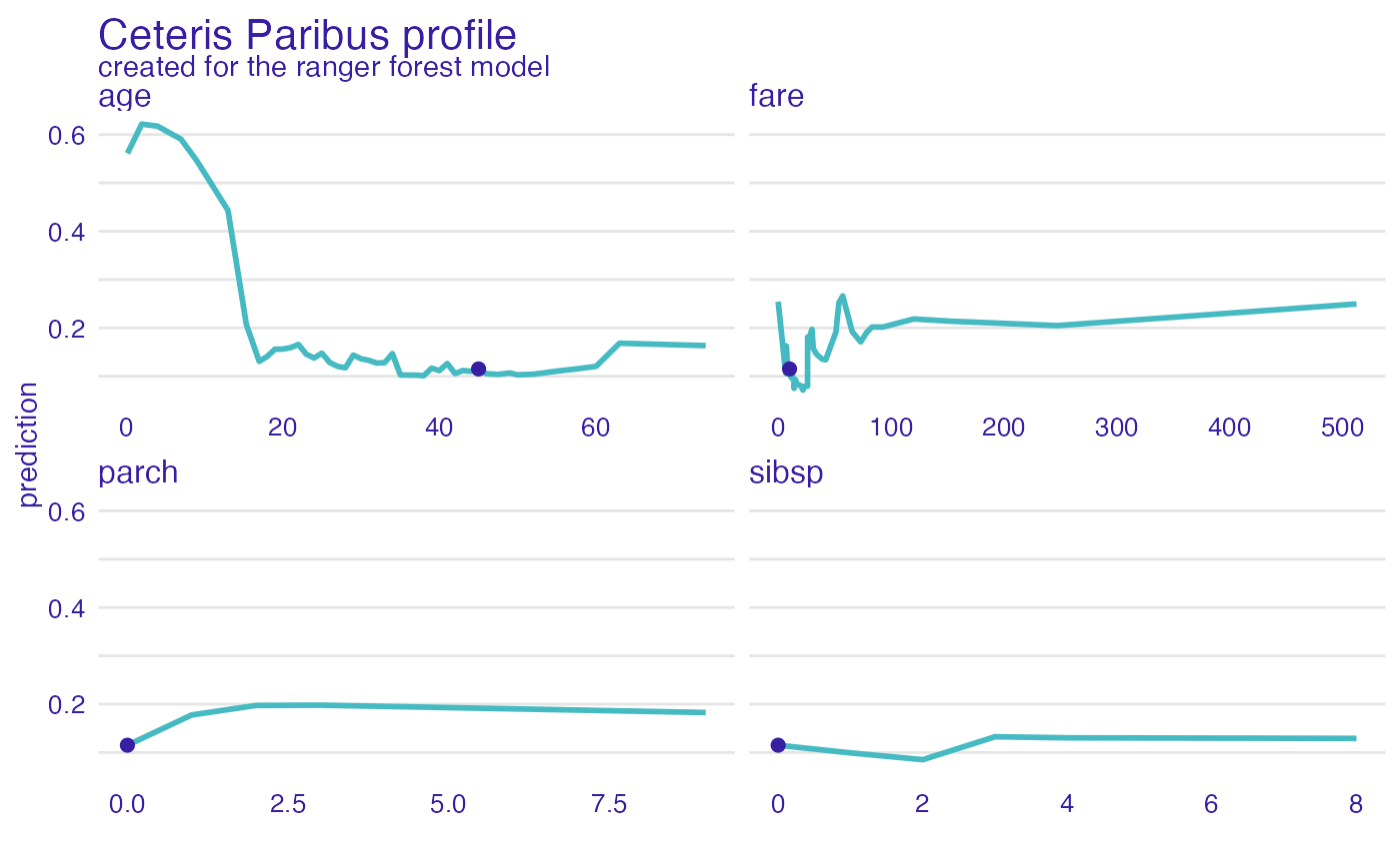
plot(cp_rf) +
show_observations(cp_rf)
selected_passangers <- select_sample(titanic_imputed, n = 1)
selected_passangers
#> gender age class embarked fare sibsp parch survived
#> 515 male 45 2nd Southampton 10.1 0 0 0
cp_rf <- ceteris_paribus(explain_titanic_rf, selected_passangers)
plot(cp_rf) +
show_observations(cp_rf)
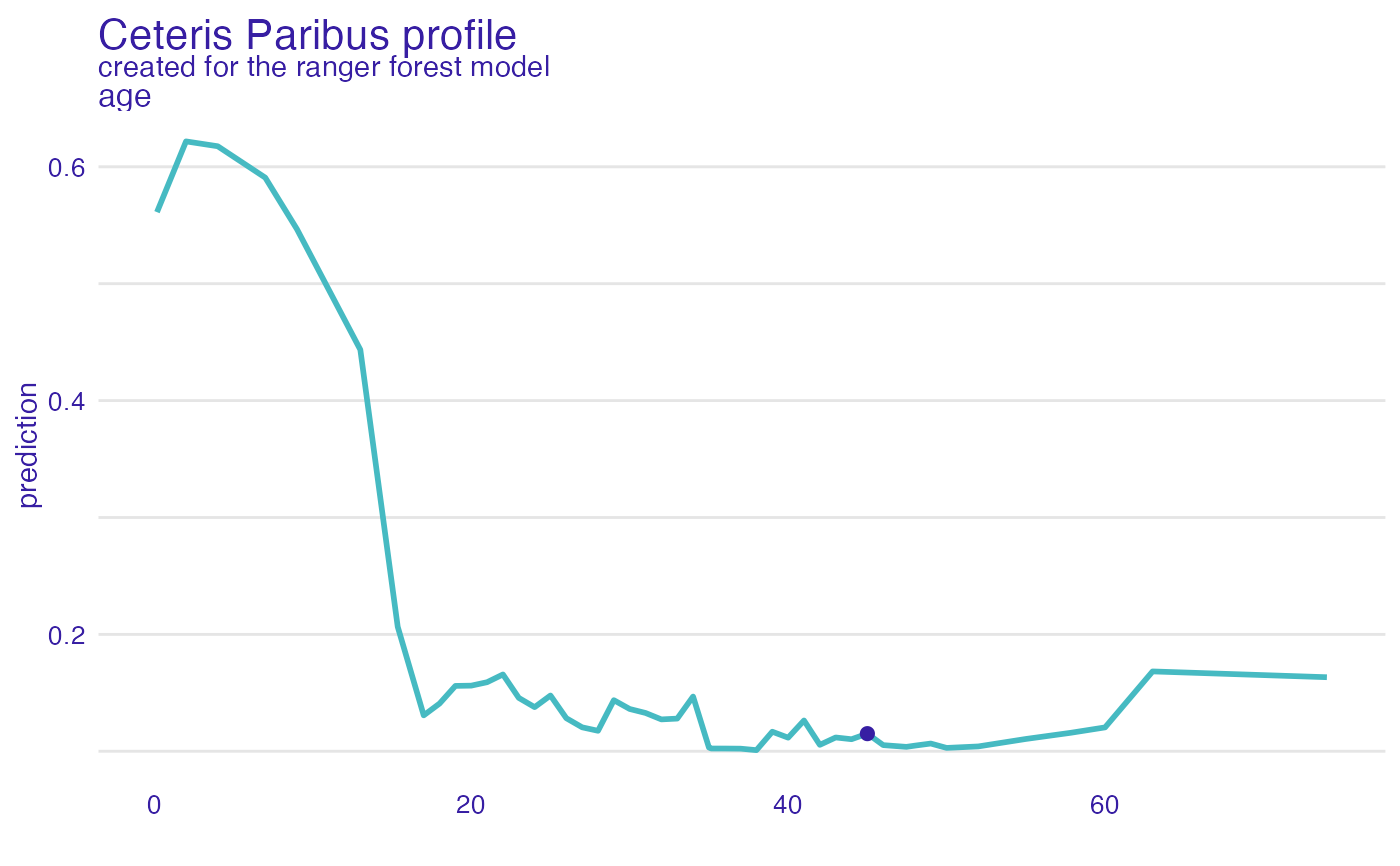
 plot(cp_rf, variables = "age") +
show_observations(cp_rf, variables = "age")
plot(cp_rf, variables = "age") +
show_observations(cp_rf, variables = "age")
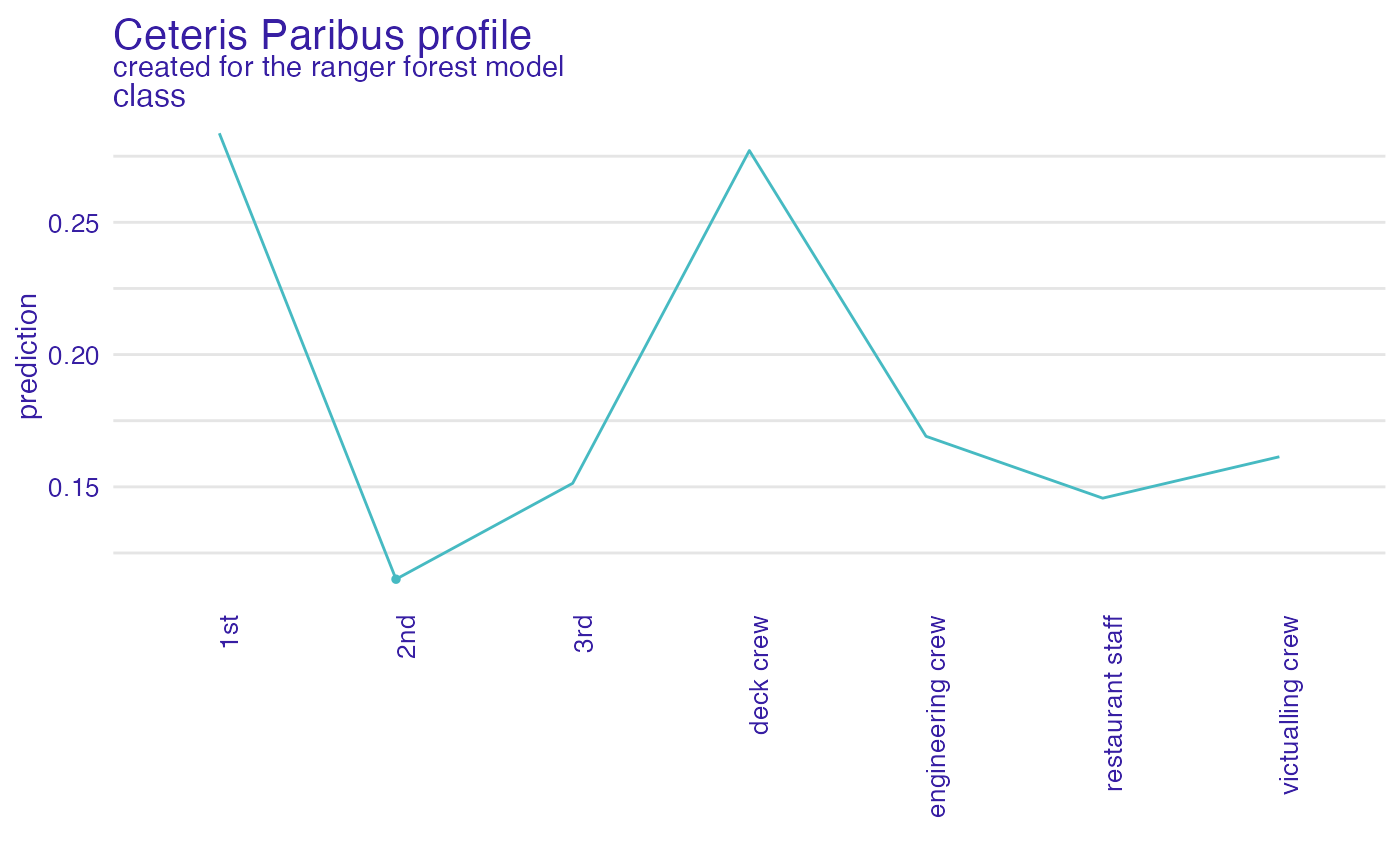
 plot(cp_rf, variables = "class")
#> 'variable_type' changed to 'categorical' due to lack of numerical variables.
plot(cp_rf, variables = "class")
#> 'variable_type' changed to 'categorical' due to lack of numerical variables.
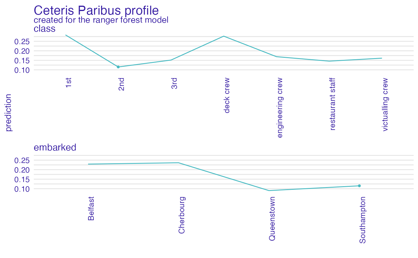
 plot(cp_rf, variables = c("class", "embarked"), facet_ncol = 1)
#> 'variable_type' changed to 'categorical' due to lack of numerical variables.
plot(cp_rf, variables = c("class", "embarked"), facet_ncol = 1)
#> 'variable_type' changed to 'categorical' due to lack of numerical variables.
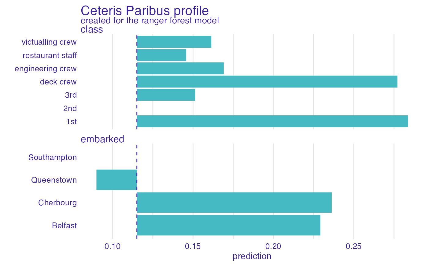
 plot(cp_rf, variables = c("class", "embarked"), facet_ncol = 1, categorical_type = "bars")
#> 'variable_type' changed to 'categorical' due to lack of numerical variables.
plot(cp_rf, variables = c("class", "embarked"), facet_ncol = 1, categorical_type = "bars")
#> 'variable_type' changed to 'categorical' due to lack of numerical variables.
 plotD3(cp_rf, variables = c("class", "embarked", "gender"),
variable_type = "categorical", scale_plot = TRUE,
label_margin = 70)
# }
plotD3(cp_rf, variables = c("class", "embarked", "gender"),
variable_type = "categorical", scale_plot = TRUE,
label_margin = 70)
# }