The function aggregate_profiles() calculates an aggregate of ceteris paribus profiles.
It can be: Partial Dependence Profile (average across Ceteris Paribus Profiles),
Conditional Dependence Profile (local weighted average across Ceteris Paribus Profiles) or
Accumulated Local Dependence Profile (cummulated average local changes in Ceteris Paribus Profiles).
aggregate_profiles(
  x,
  ...,
  variable_type = "numerical",
  groups = NULL,
  type = "partial",
  variables = NULL,
  span = 0.25,
  center = FALSE
)
Arguments
- x
a ceteris paribus explainer produced with function
ceteris_paribus()- ...
other explainers that shall be calculated together
- variable_type
a character. If
numericalthen only numerical variables will be calculated. Ifcategoricalthen only categorical variables will be calculated.- groups
a variable name that will be used for grouping. By default
NULLwhich means that no groups shall be calculated- type
either
partial/conditional/accumulatedfor partial dependence, conditional profiles of accumulated local effects- variables
if not
NULLthen aggregate only for selectedvariableswill be calculated- span
smoothing coefficient, by default
0.25. It's the sd for gaussian kernel- center
by default accumulated profiles start at 0. If
center=TRUE, then they are centered around mean prediction, which is calculated on the observations used inceteris_paribus.
Value
an object of the class aggregated_profiles_explainer
References
Explanatory Model Analysis. Explore, Explain, and Examine Predictive Models. https://ema.drwhy.ai/
Examples
library("DALEX")
library("ingredients")
library("ranger")
head(titanic_imputed)
#> gender age class embarked fare sibsp parch survived
#> 1 male 42 3rd Southampton 7.11 0 0 0
#> 2 male 13 3rd Southampton 20.05 0 2 0
#> 3 male 16 3rd Southampton 20.05 1 1 0
#> 4 female 39 3rd Southampton 20.05 1 1 1
#> 5 female 16 3rd Southampton 7.13 0 0 1
#> 6 male 25 3rd Southampton 7.13 0 0 1
# \donttest{
model_titanic_rf <- ranger(survived ~., data = titanic_imputed, probability = TRUE)
explain_titanic_rf <- explain(model_titanic_rf,
data = titanic_imputed[,-8],
y = titanic_imputed[,8],
label = "ranger forest",
verbose = FALSE)
selected_passangers <- select_sample(titanic_imputed, n = 100)
cp_rf <- ceteris_paribus(explain_titanic_rf, selected_passangers)
head(cp_rf)
#> Top profiles :
#> gender age class embarked fare sibsp parch _yhat_
#> 515 female 45 2nd Southampton 10.1000 0 0 0.8225742
#> 515.1 male 45 2nd Southampton 10.1000 0 0 0.1013317
#> 604 female 17 3rd Southampton 7.1701 1 0 0.4198725
#> 604.1 male 17 3rd Southampton 7.1701 1 0 0.1092715
#> 1430 female 25 engineering crew Southampton 0.0000 0 0 0.7558653
#> 1430.1 male 25 engineering crew Southampton 0.0000 0 0 0.2393241
#> _vname_ _ids_ _label_
#> 515 gender 515 ranger forest
#> 515.1 gender 515 ranger forest
#> 604 gender 604 ranger forest
#> 604.1 gender 604 ranger forest
#> 1430 gender 1430 ranger forest
#> 1430.1 gender 1430 ranger forest
#>
#>
#> Top observations:
#> gender age class embarked fare sibsp parch _yhat_
#> 515 male 45 2nd Southampton 10.1000 0 0 0.1013317
#> 604 male 17 3rd Southampton 7.1701 1 0 0.1092715
#> 1430 male 25 engineering crew Southampton 0.0000 0 0 0.2393241
#> 865 male 20 3rd Cherbourg 7.0406 0 0 0.1126559
#> 452 female 17 3rd Queenstown 7.1408 0 0 0.6489426
#> 1534 male 38 victualling crew Southampton 0.0000 0 0 0.1721422
#> _label_ _ids_
#> 515 ranger forest 1
#> 604 ranger forest 2
#> 1430 ranger forest 3
#> 865 ranger forest 4
#> 452 ranger forest 5
#> 1534 ranger forest 6
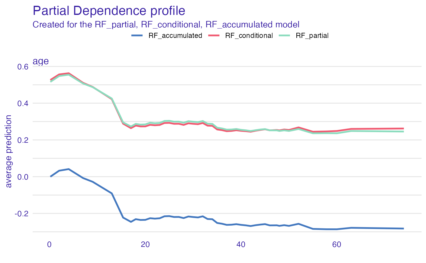
# continuous variable
pdp_rf_p <- aggregate_profiles(cp_rf, variables = "age", type = "partial")
pdp_rf_p$`_label_` <- "RF_partial"
pdp_rf_c <- aggregate_profiles(cp_rf, variables = "age", type = "conditional")
pdp_rf_c$`_label_` <- "RF_conditional"
pdp_rf_a <- aggregate_profiles(cp_rf, variables = "age", type = "accumulated")
pdp_rf_a$`_label_` <- "RF_accumulated"
plot(pdp_rf_p, pdp_rf_c, pdp_rf_a, color = "_label_")
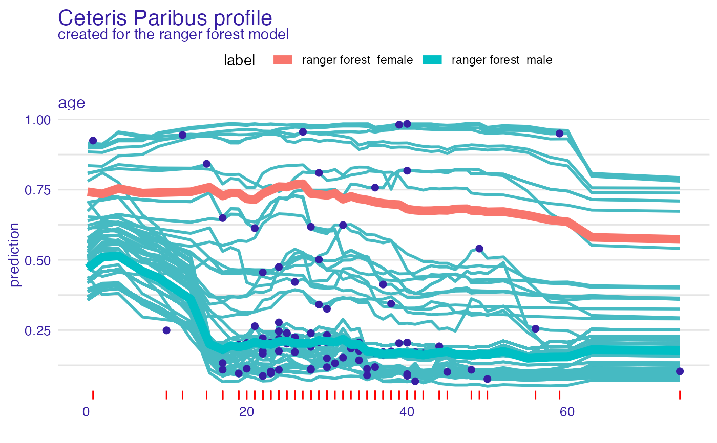
 pdp_rf <- aggregate_profiles(cp_rf, variables = "age",
groups = "gender")
head(pdp_rf)
#> Top profiles :
#> _vname_ _label_ _x_ _groups_ _yhat_ _ids_
#> 1 age ranger forest_female 0.1666667 female 0.7424940 0
#> 2 age ranger forest_female 2.0000000 female 0.7350256 0
#> 3 age ranger forest_female 4.0000000 female 0.7542271 0
#> 4 age ranger forest_female 7.0000000 female 0.7375356 0
#> 5 age ranger forest_female 9.0000000 female 0.7395428 0
#> 6 age ranger forest_female 13.0000000 female 0.7425255 0
plot(cp_rf, variables = "age") +
show_observations(cp_rf, variables = "age") +
show_rugs(cp_rf, variables = "age", color = "red") +
show_aggregated_profiles(pdp_rf, size = 3, color = "_label_")
pdp_rf <- aggregate_profiles(cp_rf, variables = "age",
groups = "gender")
head(pdp_rf)
#> Top profiles :
#> _vname_ _label_ _x_ _groups_ _yhat_ _ids_
#> 1 age ranger forest_female 0.1666667 female 0.7424940 0
#> 2 age ranger forest_female 2.0000000 female 0.7350256 0
#> 3 age ranger forest_female 4.0000000 female 0.7542271 0
#> 4 age ranger forest_female 7.0000000 female 0.7375356 0
#> 5 age ranger forest_female 9.0000000 female 0.7395428 0
#> 6 age ranger forest_female 13.0000000 female 0.7425255 0
plot(cp_rf, variables = "age") +
show_observations(cp_rf, variables = "age") +
show_rugs(cp_rf, variables = "age", color = "red") +
show_aggregated_profiles(pdp_rf, size = 3, color = "_label_")
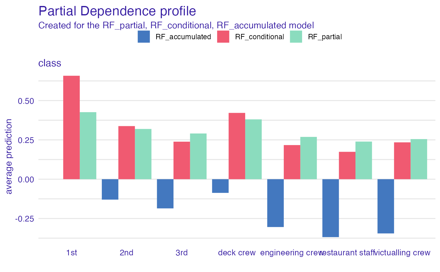
 # categorical variable
pdp_rf_p <- aggregate_profiles(cp_rf, variables = "class",
variable_type = "categorical", type = "partial")
pdp_rf_p$`_label_` <- "RF_partial"
pdp_rf_c <- aggregate_profiles(cp_rf, variables = "class",
variable_type = "categorical", type = "conditional")
pdp_rf_c$`_label_` <- "RF_conditional"
pdp_rf_a <- aggregate_profiles(cp_rf, variables = "class",
variable_type = "categorical", type = "accumulated")
pdp_rf_a$`_label_` <- "RF_accumulated"
plot(pdp_rf_p, pdp_rf_c, pdp_rf_a, color = "_label_")
# categorical variable
pdp_rf_p <- aggregate_profiles(cp_rf, variables = "class",
variable_type = "categorical", type = "partial")
pdp_rf_p$`_label_` <- "RF_partial"
pdp_rf_c <- aggregate_profiles(cp_rf, variables = "class",
variable_type = "categorical", type = "conditional")
pdp_rf_c$`_label_` <- "RF_conditional"
pdp_rf_a <- aggregate_profiles(cp_rf, variables = "class",
variable_type = "categorical", type = "accumulated")
pdp_rf_a$`_label_` <- "RF_accumulated"
plot(pdp_rf_p, pdp_rf_c, pdp_rf_a, color = "_label_")
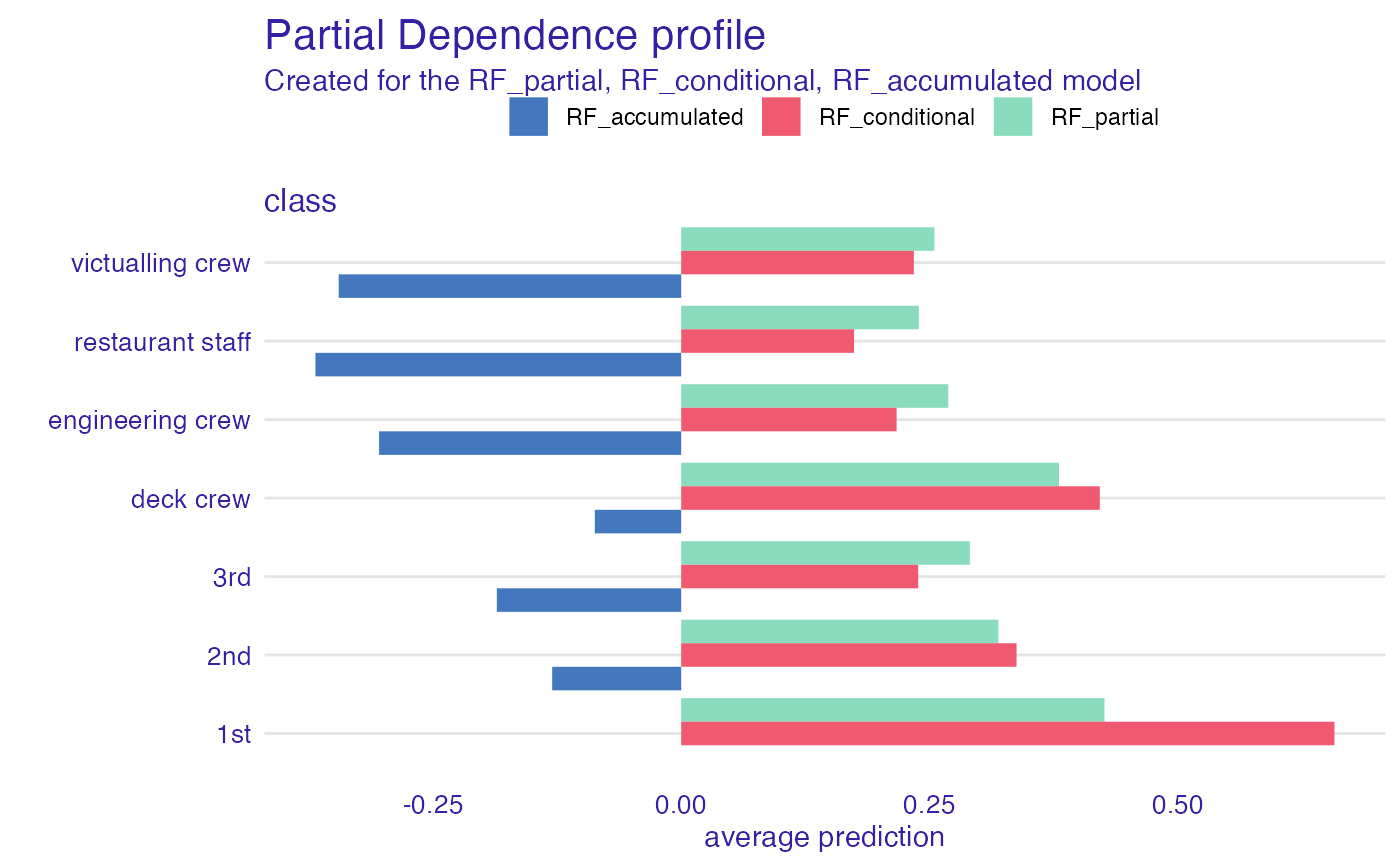
 # or maybe flipped?
library(ggplot2)
plot(pdp_rf_p, pdp_rf_c, pdp_rf_a, color = "_label_") + coord_flip()
# or maybe flipped?
library(ggplot2)
plot(pdp_rf_p, pdp_rf_c, pdp_rf_a, color = "_label_") + coord_flip()
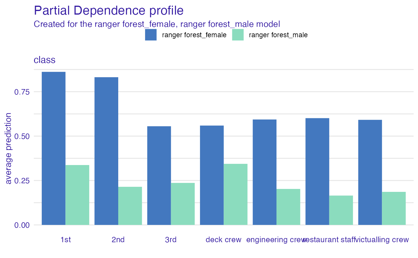
 pdp_rf <- aggregate_profiles(cp_rf, variables = "class", variable_type = "categorical",
groups = "gender")
head(pdp_rf)
#> Top profiles :
#> _vname_ _label_ _x_ _groups_ _yhat_ _ids_
#> 1 class ranger forest_female 1st female 0.8617957 0
#> 8 class ranger forest_male 1st male 0.3371083 0
#> 2 class ranger forest_female 2nd female 0.8316462 0
#> 9 class ranger forest_male 2nd male 0.2145486 0
#> 3 class ranger forest_female 3rd female 0.5555397 0
#> 10 class ranger forest_male 3rd male 0.2364858 0
plot(pdp_rf, variables = "class")
pdp_rf <- aggregate_profiles(cp_rf, variables = "class", variable_type = "categorical",
groups = "gender")
head(pdp_rf)
#> Top profiles :
#> _vname_ _label_ _x_ _groups_ _yhat_ _ids_
#> 1 class ranger forest_female 1st female 0.8617957 0
#> 8 class ranger forest_male 1st male 0.3371083 0
#> 2 class ranger forest_female 2nd female 0.8316462 0
#> 9 class ranger forest_male 2nd male 0.2145486 0
#> 3 class ranger forest_female 3rd female 0.5555397 0
#> 10 class ranger forest_male 3rd male 0.2364858 0
plot(pdp_rf, variables = "class")
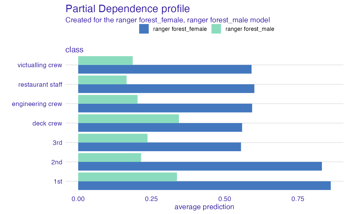
 # or maybe flipped?
plot(pdp_rf, variables = "class") + coord_flip()
# or maybe flipped?
plot(pdp_rf, variables = "class") + coord_flip()
 # }
# }