General introduction: iBreakDown plots for Sinking of the RMS Titanic

Przemyslaw Biecek

2022-02-06

Data for Titanic survival

Let’s see an example for iBreakDown plots for survival probability of Titanic passengers. First, let’s see the data, we will find quite nice data from in the DALEX package (orginally stablelearner).

library("DALEX")
head(titanic)

#>   gender age class    embarked       country  fare sibsp parch survived
#> 1   male  42   3rd Southampton United States  7.11     0     0       no
#> 2   male  13   3rd Southampton United States 20.05     0     2       no
#> 3   male  16   3rd Southampton United States 20.05     1     1       no
#> 4 female  39   3rd Southampton       England 20.05     1     1      yes
#> 5 female  16   3rd Southampton        Norway  7.13     0     0      yes
#> 6   male  25   3rd Southampton United States  7.13     0     0      yes

Model for Titanic survival

Ok, now it’s time to create a model. Let’s use the Random Forest model.

# prepare model
library("randomForest")
titanic <- na.omit(titanic)
model_titanic_rf <- randomForest(survived == "yes" ~ gender + age + class + embarked +
                                   fare + sibsp + parch,  data = titanic)
model_titanic_rf

#> 
#> Call:
#>  randomForest(formula = survived == "yes" ~ gender + age + class +      embarked + fare + sibsp + parch, data = titanic) 
#>                Type of random forest: regression
#>                      Number of trees: 500
#> No. of variables tried at each split: 2
#> 
#>           Mean of squared residuals: 0.1425301
#>                     % Var explained: 34.97

Explainer for Titanic survival

The third step (it’s optional but useful) is to create a DALEX explainer for Random Forest model.

library("DALEX")
explain_titanic_rf <- explain(model_titanic_rf, 
                      data = titanic[,-9],
                      y = titanic$survived == "yes", 
                      label = "Random Forest v7")

#> Preparation of a new explainer is initiated
#>   -> model label       :  Random Forest v7 
#>   -> data              :  2099  rows  8  cols 
#>   -> target variable   :  2099  values 
#>   -> predict function  :  yhat.randomForest  will be used (  default  )
#>   -> predicted values  :  No value for predict function target column. (  default  )
#>   -> model_info        :  package randomForest , ver. 4.7.1 , task regression (  default  ) 
#>   -> model_info        :  Model info detected regression task but 'y' is a logical .  (  WARNING  )
#>   -> model_info        :  By deafult regressions tasks supports only numercical 'y' parameter. 
#>   -> model_info        :  Consider changing to numerical vector.
#>   -> model_info        :  Otherwise I will not be able to calculate residuals or loss function.
#>   -> predicted values  :  numerical, min =  0.01000576 , mean =  0.3249614 , max =  0.9917294  
#>   -> residual function :  difference between y and yhat (  default  )
#>   -> residuals         :  numerical, min =  -0.7829437 , mean =  -0.000521225 , max =  0.8976734  
#>   A new explainer has been created! 

Break Down plot with D3

Let’s see Break Down for model predictions for 8 years old male from 1st class that embarked from port C.

new_passanger <- data.frame(
  class = factor("1st", levels = c("1st", "2nd", "3rd", "deck crew", "engineering crew", "restaurant staff", "victualling crew")),
  gender = factor("male", levels = c("female", "male")),
  age = 8,
  sibsp = 0,
  parch = 0,
  fare = 72,
  embarked = factor("Southampton", levels = c("Belfast", "Cherbourg", "Queenstown", "Southampton"))
)

Calculate variable attributions

library("iBreakDown")
rf_la <- local_attributions(explain_titanic_rf, new_passanger)
rf_la

#>                                          contribution
#> Random Forest v7: intercept                     0.325
#> Random Forest v7: age = 8                       0.221
#> Random Forest v7: class = 1st                   0.075
#> Random Forest v7: gender = male                -0.049
#> Random Forest v7: fare = 72                    -0.063
#> Random Forest v7: embarked = Southampton       -0.020
#> Random Forest v7: sibsp = 0                    -0.007
#> Random Forest v7: parch = 0                    -0.028
#> Random Forest v7: prediction                    0.455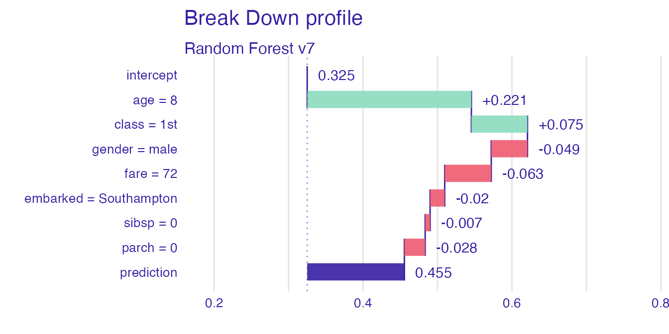

Plot attributions with ggplot2

plot(rf_la)

Plot attributions with D3

plotD3(rf_la)

Calculate uncertainty for variable attributions

rf_la_un <- break_down_uncertainty(explain_titanic_rf, new_passanger,
                         path = "average")
plot(rf_la_un)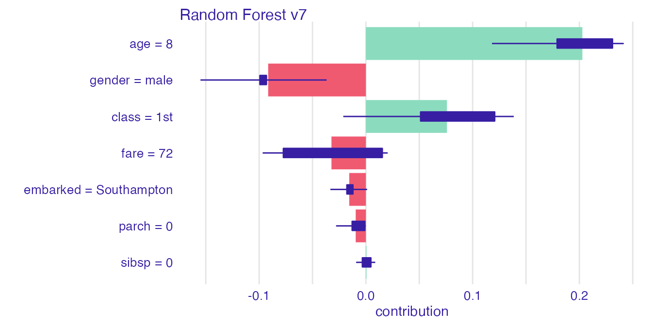

Show only top features

plotD3(rf_la, max_features = 3)

Force OX axis to be from 0 to 1

plotD3(rf_la, max_features = 3, min_max = c(0,1), margin = 0)