Model Agnostic Sequential Variable attributions
Source:R/local_attributions.R
local_attributions.RdThis function finds Variable attributions via Sequential Variable Conditioning.
The complexity of this function is O(2*p).
This function works in a similar way to step-up and step-down greedy approximations in function break_down.
The main difference is that in the first step the order of variables is determined.
And in the second step the impact is calculated.
local_attributions(x, ...)

# S3 method for explainer
local_attributions(x, new_observation, keep_distributions = FALSE, ...)

# S3 method for default
local_attributions(
  x,
  data,
  predict_function = predict,
  new_observation,
  label = class(x)[1],
  keep_distributions = FALSE,
  order = NULL,
  ...
)
Arguments
- x
an explainer created with function
explainor a model.- ...
other parameters.
- new_observation
a new observation with columns that correspond to variables used in the model.
- keep_distributions
if
TRUE, then distribution of partial predictions is stored and can be plotted with the genericplot().- data
validation dataset, will be extracted from
xif it is an explainer.- predict_function
predict function, will be extracted from
xif it is an explainer.- label
name of the model. By default it's extracted from the 'class' attribute of the model.
- order
if not
NULL, then it will be a fixed order of variables. It can be a numeric vector or vector with names of variables.
Value
an object of the break_down class.
References
Explanatory Model Analysis. Explore, Explain and Examine Predictive Models. https://ema.drwhy.ai
See also
Examples
library("DALEX")
library("iBreakDown")
set.seed(1313)
model_titanic_glm <- glm(survived ~ gender + age + fare,
data = titanic_imputed, family = "binomial")
explain_titanic_glm <- explain(model_titanic_glm,
data = titanic_imputed,
y = titanic_imputed$survived,
label = "glm")
#> Preparation of a new explainer is initiated
#> -> model label : glm
#> -> data : 2207 rows 8 cols
#> -> target variable : 2207 values
#> -> predict function : yhat.glm will be used ( default )
#> -> predicted values : No value for predict function target column. ( default )
#> -> model_info : package stats , ver. 4.1.2 , task classification ( default )
#> -> predicted values : numerical, min = 0.1490412 , mean = 0.3221568 , max = 0.9878987
#> -> residual function : difference between y and yhat ( default )
#> -> residuals : numerical, min = -0.8898433 , mean = 4.198546e-13 , max = 0.8448637
#> A new explainer has been created!
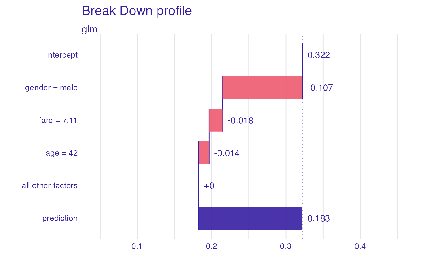
bd_glm <- local_attributions(explain_titanic_glm, titanic_imputed[1, ])
bd_glm
#> contribution
#> glm: intercept 0.322
#> glm: gender = male -0.107
#> glm: fare = 7.11 -0.018
#> glm: age = 42 -0.014
#> glm: class = 3rd 0.000
#> glm: embarked = Southampton 0.000
#> glm: sibsp = 0 0.000
#> glm: parch = 0 0.000
#> glm: survived = 0 0.000
#> glm: prediction 0.183
plot(bd_glm, max_features = 3)
 # \dontrun{
## Not run:
library("randomForest")
set.seed(1313)
# example with interaction
# classification for HR data
model <- randomForest(status ~ . , data = HR)
new_observation <- HR_test[1,]
explainer_rf <- explain(model,
data = HR[1:1000,1:5])
#> Preparation of a new explainer is initiated
#> -> model label : randomForest ( default )
#> -> data : 1000 rows 5 cols
#> -> target variable : not specified! ( WARNING )
#> -> predict function : yhat.randomForest will be used ( default )
#> -> predicted values : No value for predict function target column. ( default )
#> -> model_info : package randomForest , ver. 4.7.1 , task multiclass ( default )
#> -> model_info : Model info detected multiclass task but 'y' is a NULL . ( WARNING )
#> -> model_info : By deafult multiclass tasks supports only factor 'y' parameter.
#> -> model_info : Consider changing to a factor vector with true class names.
#> -> model_info : Otherwise I will not be able to calculate residuals or loss function.
#> -> predicted values : predict function returns multiple columns: 3 ( default )
#> -> residual function : difference between 1 and probability of true class ( default )
#> A new explainer has been created!
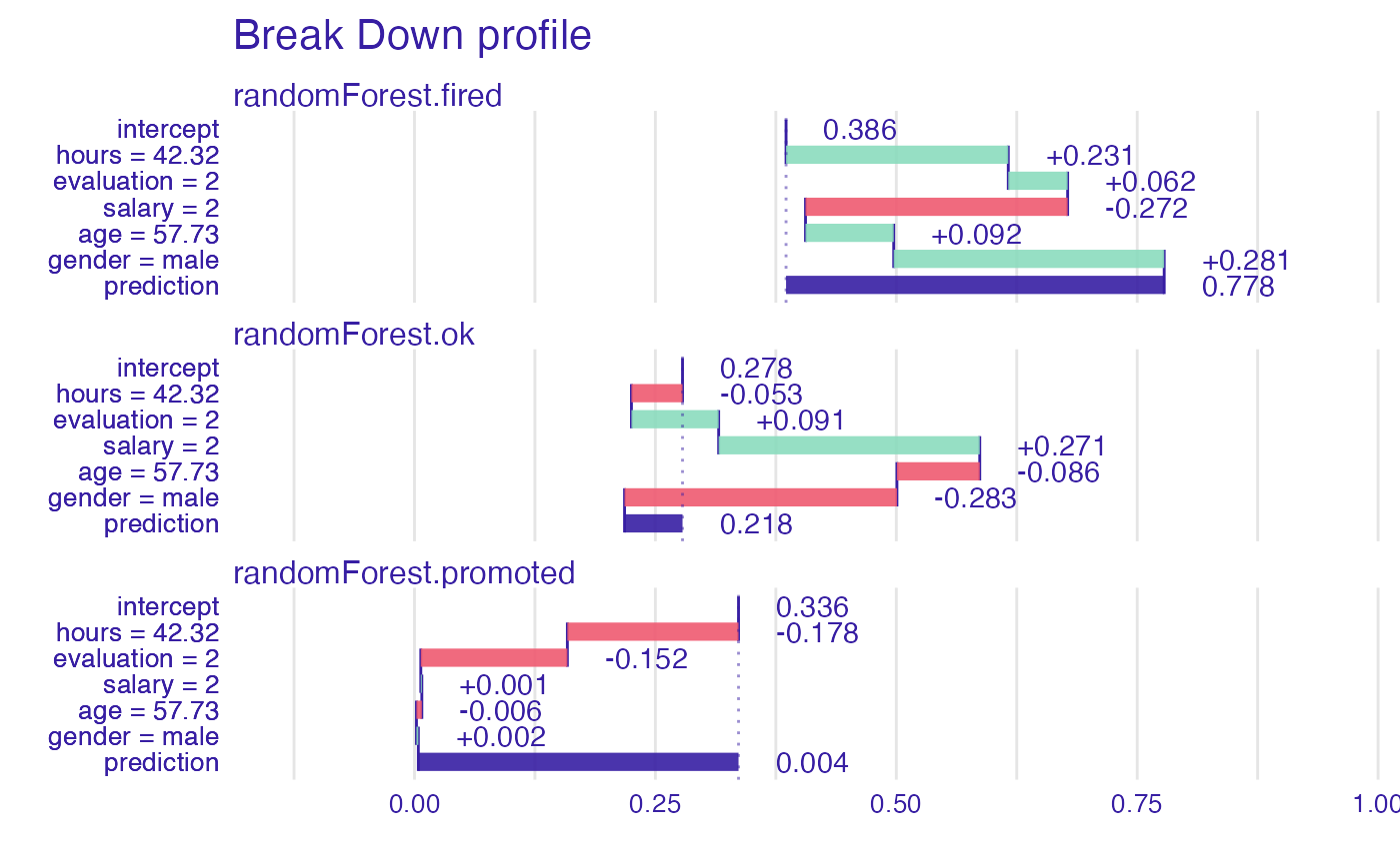
bd_rf <- local_attributions(explainer_rf,
new_observation)
bd_rf
#> contribution
#> randomForest.fired: intercept 0.386
#> randomForest.fired: hours = 42.32 0.231
#> randomForest.fired: evaluation = 2 0.062
#> randomForest.fired: salary = 2 -0.272
#> randomForest.fired: age = 57.73 0.092
#> randomForest.fired: gender = male 0.281
#> randomForest.fired: prediction 0.778
#> randomForest.ok: intercept 0.278
#> randomForest.ok: hours = 42.32 -0.053
#> randomForest.ok: evaluation = 2 0.091
#> randomForest.ok: salary = 2 0.271
#> randomForest.ok: age = 57.73 -0.086
#> randomForest.ok: gender = male -0.283
#> randomForest.ok: prediction 0.218
#> randomForest.promoted: intercept 0.336
#> randomForest.promoted: hours = 42.32 -0.178
#> randomForest.promoted: evaluation = 2 -0.152
#> randomForest.promoted: salary = 2 0.001
#> randomForest.promoted: age = 57.73 -0.006
#> randomForest.promoted: gender = male 0.002
#> randomForest.promoted: prediction 0.004
plot(bd_rf)
# \dontrun{
## Not run:
library("randomForest")
set.seed(1313)
# example with interaction
# classification for HR data
model <- randomForest(status ~ . , data = HR)
new_observation <- HR_test[1,]
explainer_rf <- explain(model,
data = HR[1:1000,1:5])
#> Preparation of a new explainer is initiated
#> -> model label : randomForest ( default )
#> -> data : 1000 rows 5 cols
#> -> target variable : not specified! ( WARNING )
#> -> predict function : yhat.randomForest will be used ( default )
#> -> predicted values : No value for predict function target column. ( default )
#> -> model_info : package randomForest , ver. 4.7.1 , task multiclass ( default )
#> -> model_info : Model info detected multiclass task but 'y' is a NULL . ( WARNING )
#> -> model_info : By deafult multiclass tasks supports only factor 'y' parameter.
#> -> model_info : Consider changing to a factor vector with true class names.
#> -> model_info : Otherwise I will not be able to calculate residuals or loss function.
#> -> predicted values : predict function returns multiple columns: 3 ( default )
#> -> residual function : difference between 1 and probability of true class ( default )
#> A new explainer has been created!
bd_rf <- local_attributions(explainer_rf,
new_observation)
bd_rf
#> contribution
#> randomForest.fired: intercept 0.386
#> randomForest.fired: hours = 42.32 0.231
#> randomForest.fired: evaluation = 2 0.062
#> randomForest.fired: salary = 2 -0.272
#> randomForest.fired: age = 57.73 0.092
#> randomForest.fired: gender = male 0.281
#> randomForest.fired: prediction 0.778
#> randomForest.ok: intercept 0.278
#> randomForest.ok: hours = 42.32 -0.053
#> randomForest.ok: evaluation = 2 0.091
#> randomForest.ok: salary = 2 0.271
#> randomForest.ok: age = 57.73 -0.086
#> randomForest.ok: gender = male -0.283
#> randomForest.ok: prediction 0.218
#> randomForest.promoted: intercept 0.336
#> randomForest.promoted: hours = 42.32 -0.178
#> randomForest.promoted: evaluation = 2 -0.152
#> randomForest.promoted: salary = 2 0.001
#> randomForest.promoted: age = 57.73 -0.006
#> randomForest.promoted: gender = male 0.002
#> randomForest.promoted: prediction 0.004
plot(bd_rf)
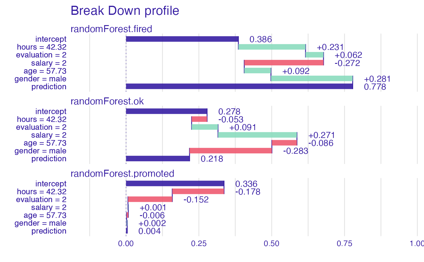
 plot(bd_rf, baseline = 0)
 # example for regression - apartment prices
# here we do not have interactions
model <- randomForest(m2.price ~ . , data = apartments)
explainer_rf <- explain(model,
data = apartments_test[1:1000,2:6],
y = apartments_test$m2.price[1:1000])
#> Preparation of a new explainer is initiated
#> -> model label : randomForest ( default )
#> -> data : 1000 rows 5 cols
#> -> target variable : 1000 values
#> -> predict function : yhat.randomForest will be used ( default )
#> -> predicted values : No value for predict function target column. ( default )
#> -> model_info : package randomForest , ver. 4.7.1 , task regression ( default )
#> -> predicted values : numerical, min = 2043.066 , mean = 3487.722 , max = 5773.976
#> -> residual function : difference between y and yhat ( default )
#> -> residuals : numerical, min = -630.6766 , mean = 1.057813 , max = 1256.239
#> A new explainer has been created!
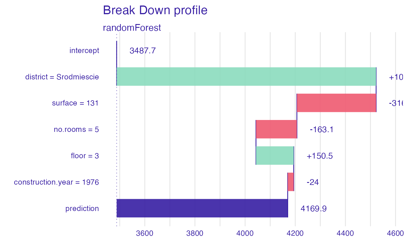
bd_rf <- local_attributions(explainer_rf,
apartments_test[1,])
bd_rf
#> contribution
#> randomForest: intercept 3487.722
#> randomForest: district = Srodmiescie 1034.737
#> randomForest: surface = 131 -315.991
#> randomForest: no.rooms = 5 -163.113
#> randomForest: floor = 3 150.529
#> randomForest: construction.year = 1976 -24.021
#> randomForest: prediction 4169.863
plot(bd_rf, digits = 1)
# example for regression - apartment prices
# here we do not have interactions
model <- randomForest(m2.price ~ . , data = apartments)
explainer_rf <- explain(model,
data = apartments_test[1:1000,2:6],
y = apartments_test$m2.price[1:1000])
#> Preparation of a new explainer is initiated
#> -> model label : randomForest ( default )
#> -> data : 1000 rows 5 cols
#> -> target variable : 1000 values
#> -> predict function : yhat.randomForest will be used ( default )
#> -> predicted values : No value for predict function target column. ( default )
#> -> model_info : package randomForest , ver. 4.7.1 , task regression ( default )
#> -> predicted values : numerical, min = 2043.066 , mean = 3487.722 , max = 5773.976
#> -> residual function : difference between y and yhat ( default )
#> -> residuals : numerical, min = -630.6766 , mean = 1.057813 , max = 1256.239
#> A new explainer has been created!
bd_rf <- local_attributions(explainer_rf,
apartments_test[1,])
bd_rf
#> contribution
#> randomForest: intercept 3487.722
#> randomForest: district = Srodmiescie 1034.737
#> randomForest: surface = 131 -315.991
#> randomForest: no.rooms = 5 -163.113
#> randomForest: floor = 3 150.529
#> randomForest: construction.year = 1976 -24.021
#> randomForest: prediction 4169.863
plot(bd_rf, digits = 1)
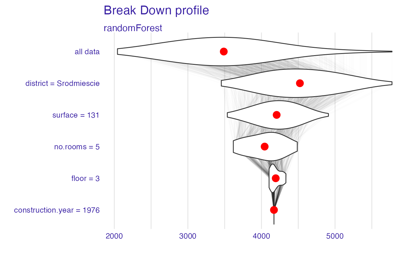
 bd_rf <- local_attributions(explainer_rf,
apartments_test[1,],
keep_distributions = TRUE)
plot(bd_rf, plot_distributions = TRUE)
#> Warning: `fun.y` is deprecated. Use `fun` instead.
bd_rf <- local_attributions(explainer_rf,
apartments_test[1,],
keep_distributions = TRUE)
plot(bd_rf, plot_distributions = TRUE)
#> Warning: `fun.y` is deprecated. Use `fun` instead.
 # }
# }