Explanation Level Uncertainty of Sequential Variable Attribution
Source:R/break_down_uncertainty.R
break_down_uncertainty.RdThis function calculates the break down algorithm for B random orderings.
Then it calculates the distribution of attributions for these different orderings.
Note that the shap() function is just a simplified interface to the break_down_uncertainty() function
with a default value set to B=25.
break_down_uncertainty(x, ..., keep_distributions = TRUE, B = 10)

# S3 method for explainer
break_down_uncertainty(
  x,
  new_observation,
  ...,
  keep_distributions = TRUE,
  B = 10
)

# S3 method for default
break_down_uncertainty(
  x,
  data,
  predict_function = predict,
  new_observation,
  label = class(x)[1],
  ...,
  path = NULL,
  keep_distributions = TRUE,
  B = 10
)

shap(x, ..., B = 25)
Arguments
- x
an explainer created with function
explainor a model.- ...
other parameters.
- keep_distributions
if
TRUEthen we will keep distribution for predicted values. It's needed by the describe function.- B
number of random paths
- new_observation
a new observation with columns that correspond to variables used in the model.
- data
validation dataset, will be extracted from
xif it is an explainer.- predict_function
predict function, will be extracted from
xif it is an explainer.- label
name of the model. By default it's extracted from the 'class' attribute of the model.
- path
if specified, then this path will be highlighed on the plot. Use
averagein order to show an average effect
Value
an object of the break_down_uncertainty class.
References
Explanatory Model Analysis. Explore, Explain and Examine Predictive Models. https://ema.drwhy.ai
See also
Examples
library("DALEX")
library("iBreakDown")
set.seed(1313)
model_titanic_glm <- glm(survived ~ gender + age + fare,
data = titanic_imputed, family = "binomial")
explain_titanic_glm <- explain(model_titanic_glm,
data = titanic_imputed,
y = titanic_imputed$survived,
label = "glm")
#> Preparation of a new explainer is initiated
#> -> model label : glm
#> -> data : 2207 rows 8 cols
#> -> target variable : 2207 values
#> -> predict function : yhat.glm will be used ( default )
#> -> predicted values : No value for predict function target column. ( default )
#> -> model_info : package stats , ver. 4.1.2 , task classification ( default )
#> -> predicted values : numerical, min = 0.1490412 , mean = 0.3221568 , max = 0.9878987
#> -> residual function : difference between y and yhat ( default )
#> -> residuals : numerical, min = -0.8898433 , mean = 4.198546e-13 , max = 0.8448637
#> A new explainer has been created!
# there is no explanation level uncertanity linked with additive models
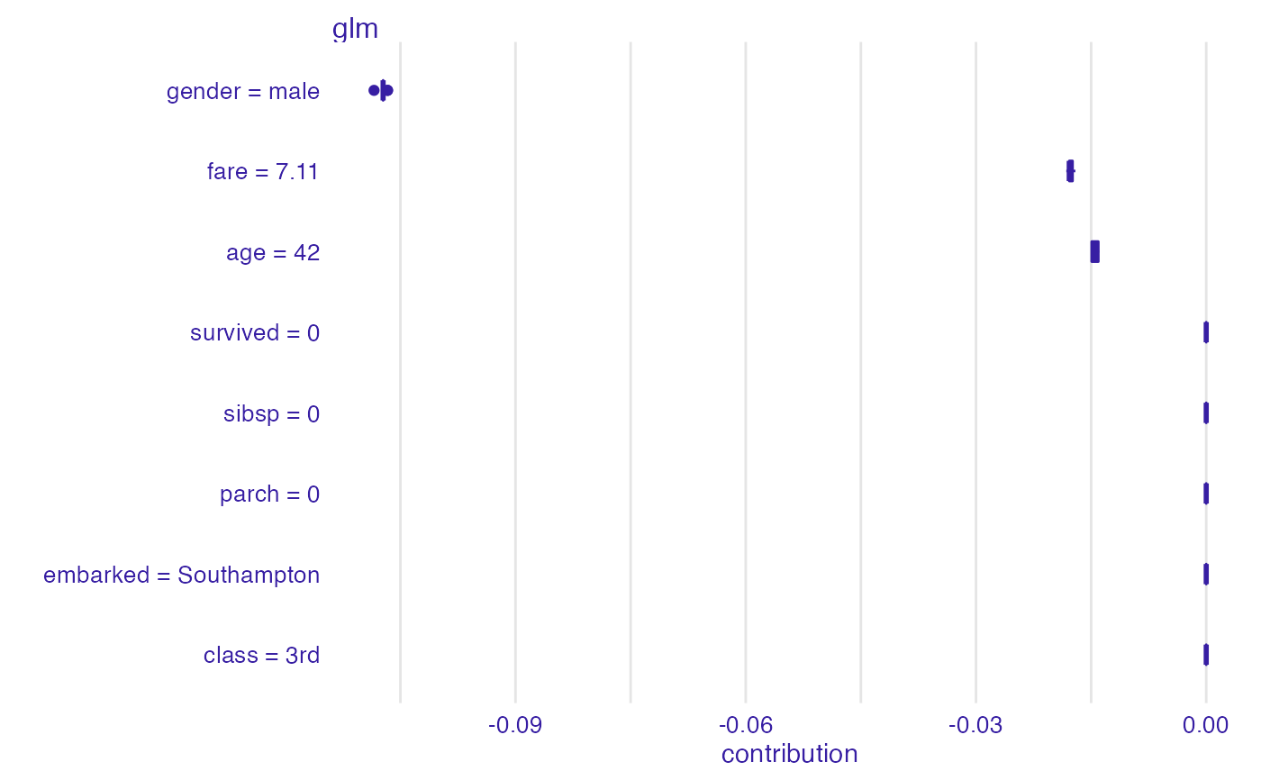
bd_glm <- break_down_uncertainty(explain_titanic_glm, titanic_imputed[1, ])
bd_glm
#> min q1 median mean
#> glm: age = 42 -0.01492541 -0.01492541 -0.01434645 -0.01446344
#> glm: class = 3rd 0.00000000 0.00000000 0.00000000 0.00000000
#> glm: embarked = Southampton 0.00000000 0.00000000 0.00000000 0.00000000
#> glm: fare = 7.11 -0.01823177 -0.01784977 -0.01784977 -0.01773120
#> glm: gender = male -0.10843751 -0.10725651 -0.10725651 -0.10725810
#> glm: parch = 0 0.00000000 0.00000000 0.00000000 0.00000000
#> glm: sibsp = 0 0.00000000 0.00000000 0.00000000 0.00000000
#> glm: survived = 0 0.00000000 0.00000000 0.00000000 0.00000000
#> q3 max
#> glm: age = 42 -0.01405996 -0.01396446
#> glm: class = 3rd 0.00000000 0.00000000
#> glm: embarked = Southampton 0.00000000 0.00000000
#> glm: fare = 7.11 -0.01741824 -0.01705077
#> glm: gender = male -0.10725293 -0.10667755
#> glm: parch = 0 0.00000000 0.00000000
#> glm: sibsp = 0 0.00000000 0.00000000
#> glm: survived = 0 0.00000000 0.00000000
plot(bd_glm)
 # \dontrun{
## Not run:
library("randomForest")
set.seed(1313)
model <- randomForest(status ~ . , data = HR)
new_observation <- HR_test[1,]
explainer_rf <- explain(model,
data = HR[1:1000, 1:5])
#> Preparation of a new explainer is initiated
#> -> model label : randomForest ( default )
#> -> data : 1000 rows 5 cols
#> -> target variable : not specified! ( WARNING )
#> -> predict function : yhat.randomForest will be used ( default )
#> -> predicted values : No value for predict function target column. ( default )
#> -> model_info : package randomForest , ver. 4.7.1 , task multiclass ( default )
#> -> model_info : Model info detected multiclass task but 'y' is a NULL . ( WARNING )
#> -> model_info : By deafult multiclass tasks supports only factor 'y' parameter.
#> -> model_info : Consider changing to a factor vector with true class names.
#> -> model_info : Otherwise I will not be able to calculate residuals or loss function.
#> -> predicted values : predict function returns multiple columns: 3 ( default )
#> -> residual function : difference between 1 and probability of true class ( default )
#> A new explainer has been created!
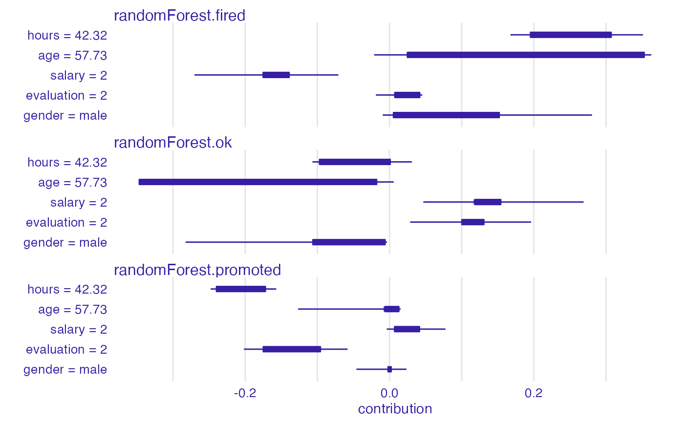
bd_rf <- break_down_uncertainty(explainer_rf,
new_observation)
bd_rf
#> min q1 median mean
#> randomForest.fired: age = 57.73 -0.021328 0.0247710 0.253395 0.1946016
#> randomForest.fired: evaluation = 2 -0.018856 0.0073270 0.032725 0.0216108
#> randomForest.fired: gender = male -0.009380 0.0054740 0.019250 0.0911182
#> randomForest.fired: hours = 42.32 0.167650 0.1953890 0.220689 0.2461712
#> randomForest.fired: salary = 2 -0.270298 -0.1751675 -0.160058 -0.1610878
#> randomForest.ok: age = 57.73 -0.346842 -0.3468420 -0.199269 -0.1834688
#> randomForest.ok: evaluation = 2 0.028666 0.1002960 0.125760 0.1215018
#> randomForest.ok: gender = male -0.282642 -0.1062540 -0.021756 -0.0845928
#> randomForest.ok: hours = 42.32 -0.106876 -0.0970580 -0.046824 -0.0447352
#> randomForest.ok: salary = 2 0.046824 0.1184785 0.118552 0.1311450
#> randomForest.promoted: age = 57.73 -0.126732 -0.0061320 -0.006132 -0.0111328
#> randomForest.promoted: evaluation = 2 -0.201822 -0.1749640 -0.166262 -0.1431126
#> randomForest.promoted: gender = male -0.045880 -0.0019940 -0.000019 -0.0065254
#> randomForest.promoted: hours = 42.32 -0.247972 -0.2398625 -0.189205 -0.2014360
#> randomForest.promoted: salary = 2 -0.003902 0.0069900 0.034329 0.0299428
#> q3 max
#> randomForest.fired: age = 57.73 0.3529740 0.362800
#> randomForest.fired: evaluation = 2 0.0418870 0.045408
#> randomForest.fired: gender = male 0.1521340 0.280686
#> randomForest.fired: hours = 42.32 0.3072255 0.351330
#> randomForest.fired: salary = 2 -0.1390850 -0.070866
#> randomForest.ok: age = 57.73 -0.0178415 0.005860
#> randomForest.ok: evaluation = 2 0.1307830 0.196252
#> randomForest.ok: gender = male -0.0061560 -0.003480
#> randomForest.ok: hours = 42.32 0.0010015 0.030996
#> randomForest.ok: salary = 2 0.1542220 0.268992
#> randomForest.promoted: age = 57.73 0.0129425 0.015468
#> randomForest.promoted: evaluation = 2 -0.0957510 -0.058120
#> randomForest.promoted: gender = male 0.0023685 0.023564
#> randomForest.promoted: hours = 42.32 -0.1719955 -0.156930
#> randomForest.promoted: salary = 2 0.0415060 0.077562
plot(bd_rf)
# \dontrun{
## Not run:
library("randomForest")
set.seed(1313)
model <- randomForest(status ~ . , data = HR)
new_observation <- HR_test[1,]
explainer_rf <- explain(model,
data = HR[1:1000, 1:5])
#> Preparation of a new explainer is initiated
#> -> model label : randomForest ( default )
#> -> data : 1000 rows 5 cols
#> -> target variable : not specified! ( WARNING )
#> -> predict function : yhat.randomForest will be used ( default )
#> -> predicted values : No value for predict function target column. ( default )
#> -> model_info : package randomForest , ver. 4.7.1 , task multiclass ( default )
#> -> model_info : Model info detected multiclass task but 'y' is a NULL . ( WARNING )
#> -> model_info : By deafult multiclass tasks supports only factor 'y' parameter.
#> -> model_info : Consider changing to a factor vector with true class names.
#> -> model_info : Otherwise I will not be able to calculate residuals or loss function.
#> -> predicted values : predict function returns multiple columns: 3 ( default )
#> -> residual function : difference between 1 and probability of true class ( default )
#> A new explainer has been created!
bd_rf <- break_down_uncertainty(explainer_rf,
new_observation)
bd_rf
#> min q1 median mean
#> randomForest.fired: age = 57.73 -0.021328 0.0247710 0.253395 0.1946016
#> randomForest.fired: evaluation = 2 -0.018856 0.0073270 0.032725 0.0216108
#> randomForest.fired: gender = male -0.009380 0.0054740 0.019250 0.0911182
#> randomForest.fired: hours = 42.32 0.167650 0.1953890 0.220689 0.2461712
#> randomForest.fired: salary = 2 -0.270298 -0.1751675 -0.160058 -0.1610878
#> randomForest.ok: age = 57.73 -0.346842 -0.3468420 -0.199269 -0.1834688
#> randomForest.ok: evaluation = 2 0.028666 0.1002960 0.125760 0.1215018
#> randomForest.ok: gender = male -0.282642 -0.1062540 -0.021756 -0.0845928
#> randomForest.ok: hours = 42.32 -0.106876 -0.0970580 -0.046824 -0.0447352
#> randomForest.ok: salary = 2 0.046824 0.1184785 0.118552 0.1311450
#> randomForest.promoted: age = 57.73 -0.126732 -0.0061320 -0.006132 -0.0111328
#> randomForest.promoted: evaluation = 2 -0.201822 -0.1749640 -0.166262 -0.1431126
#> randomForest.promoted: gender = male -0.045880 -0.0019940 -0.000019 -0.0065254
#> randomForest.promoted: hours = 42.32 -0.247972 -0.2398625 -0.189205 -0.2014360
#> randomForest.promoted: salary = 2 -0.003902 0.0069900 0.034329 0.0299428
#> q3 max
#> randomForest.fired: age = 57.73 0.3529740 0.362800
#> randomForest.fired: evaluation = 2 0.0418870 0.045408
#> randomForest.fired: gender = male 0.1521340 0.280686
#> randomForest.fired: hours = 42.32 0.3072255 0.351330
#> randomForest.fired: salary = 2 -0.1390850 -0.070866
#> randomForest.ok: age = 57.73 -0.0178415 0.005860
#> randomForest.ok: evaluation = 2 0.1307830 0.196252
#> randomForest.ok: gender = male -0.0061560 -0.003480
#> randomForest.ok: hours = 42.32 0.0010015 0.030996
#> randomForest.ok: salary = 2 0.1542220 0.268992
#> randomForest.promoted: age = 57.73 0.0129425 0.015468
#> randomForest.promoted: evaluation = 2 -0.0957510 -0.058120
#> randomForest.promoted: gender = male 0.0023685 0.023564
#> randomForest.promoted: hours = 42.32 -0.1719955 -0.156930
#> randomForest.promoted: salary = 2 0.0415060 0.077562
plot(bd_rf)
 # example for regression - apartment prices
# here we do not have intreactions
model <- randomForest(m2.price ~ . , data = apartments)
explainer_rf <- explain(model,
data = apartments_test[1:1000, 2:6],
y = apartments_test$m2.price[1:1000])
#> Preparation of a new explainer is initiated
#> -> model label : randomForest ( default )
#> -> data : 1000 rows 5 cols
#> -> target variable : 1000 values
#> -> predict function : yhat.randomForest will be used ( default )
#> -> predicted values : No value for predict function target column. ( default )
#> -> model_info : package randomForest , ver. 4.7.1 , task regression ( default )
#> -> predicted values : numerical, min = 2052.033 , mean = 3487.71 , max = 5776.623
#> -> residual function : difference between y and yhat ( default )
#> -> residuals : numerical, min = -632.8469 , mean = 1.070017 , max = 1328.352
#> A new explainer has been created!
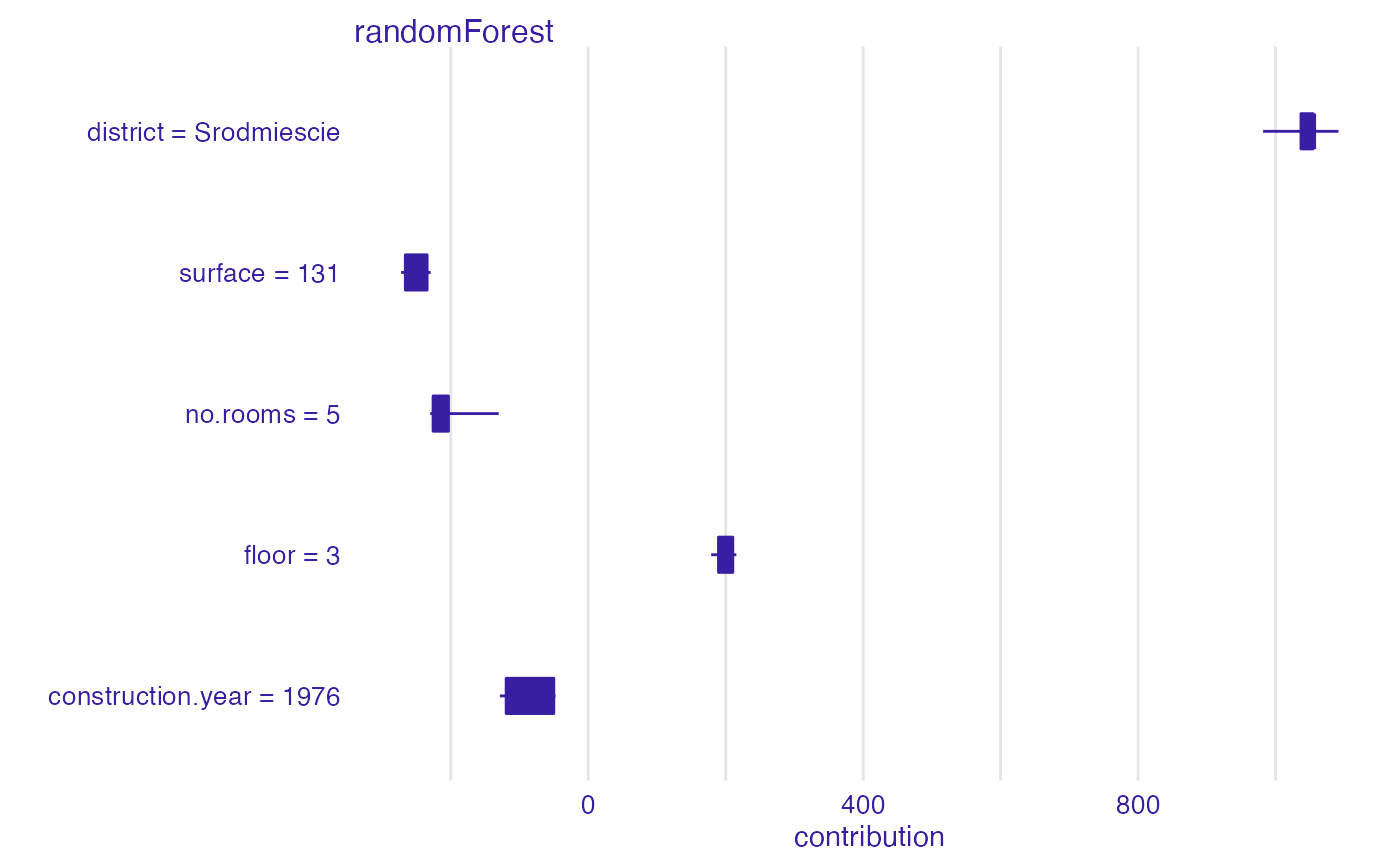
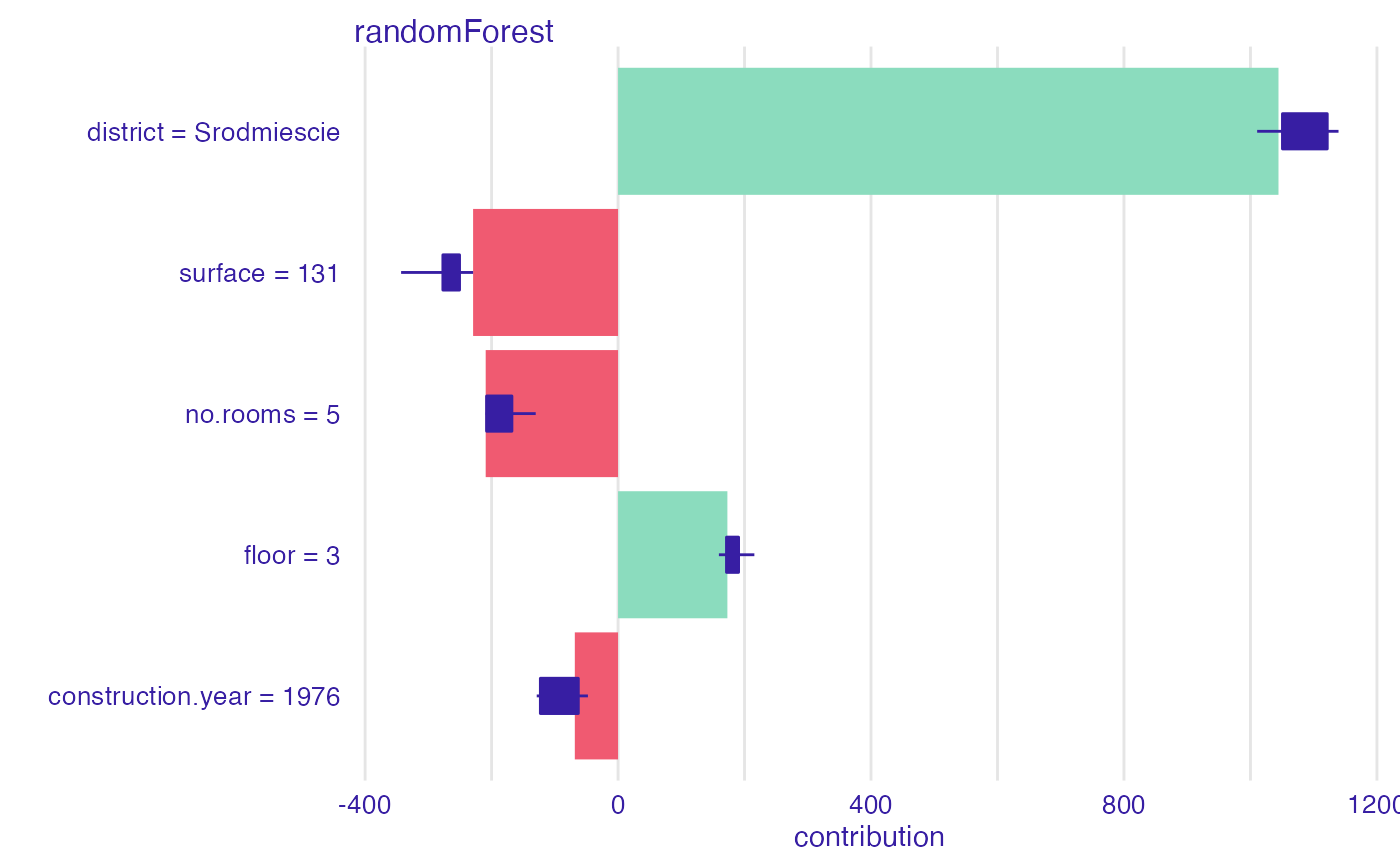
bd_rf <- break_down_uncertainty(explainer_rf, apartments_test[1,])
bd_rf
#> min q1 median
#> randomForest: construction.year = 1976 -128.5908 -119.3910 -75.48837
#> randomForest: district = Srodmiescie 981.8193 1036.9753 1054.79081
#> randomForest: floor = 3 178.8471 189.5230 194.12751
#> randomForest: no.rooms = 5 -229.8610 -225.7194 -212.31243
#> randomForest: surface = 131 -272.2211 -266.0785 -250.70512
#> mean q3 max
#> randomForest: construction.year = 1976 -82.87975 -50.06424 -47.64365
#> randomForest: district = Srodmiescie 1046.73182 1054.79081 1091.59037
#> randomForest: floor = 3 197.65920 210.33113 215.52532
#> randomForest: no.rooms = 5 -200.17988 -203.34626 -130.21186
#> randomForest: surface = 131 -250.99715 -234.39585 -229.21426
plot(bd_rf)
# example for regression - apartment prices
# here we do not have intreactions
model <- randomForest(m2.price ~ . , data = apartments)
explainer_rf <- explain(model,
data = apartments_test[1:1000, 2:6],
y = apartments_test$m2.price[1:1000])
#> Preparation of a new explainer is initiated
#> -> model label : randomForest ( default )
#> -> data : 1000 rows 5 cols
#> -> target variable : 1000 values
#> -> predict function : yhat.randomForest will be used ( default )
#> -> predicted values : No value for predict function target column. ( default )
#> -> model_info : package randomForest , ver. 4.7.1 , task regression ( default )
#> -> predicted values : numerical, min = 2052.033 , mean = 3487.71 , max = 5776.623
#> -> residual function : difference between y and yhat ( default )
#> -> residuals : numerical, min = -632.8469 , mean = 1.070017 , max = 1328.352
#> A new explainer has been created!
bd_rf <- break_down_uncertainty(explainer_rf, apartments_test[1,])
bd_rf
#> min q1 median
#> randomForest: construction.year = 1976 -128.5908 -119.3910 -75.48837
#> randomForest: district = Srodmiescie 981.8193 1036.9753 1054.79081
#> randomForest: floor = 3 178.8471 189.5230 194.12751
#> randomForest: no.rooms = 5 -229.8610 -225.7194 -212.31243
#> randomForest: surface = 131 -272.2211 -266.0785 -250.70512
#> mean q3 max
#> randomForest: construction.year = 1976 -82.87975 -50.06424 -47.64365
#> randomForest: district = Srodmiescie 1046.73182 1054.79081 1091.59037
#> randomForest: floor = 3 197.65920 210.33113 215.52532
#> randomForest: no.rooms = 5 -200.17988 -203.34626 -130.21186
#> randomForest: surface = 131 -250.99715 -234.39585 -229.21426
plot(bd_rf)
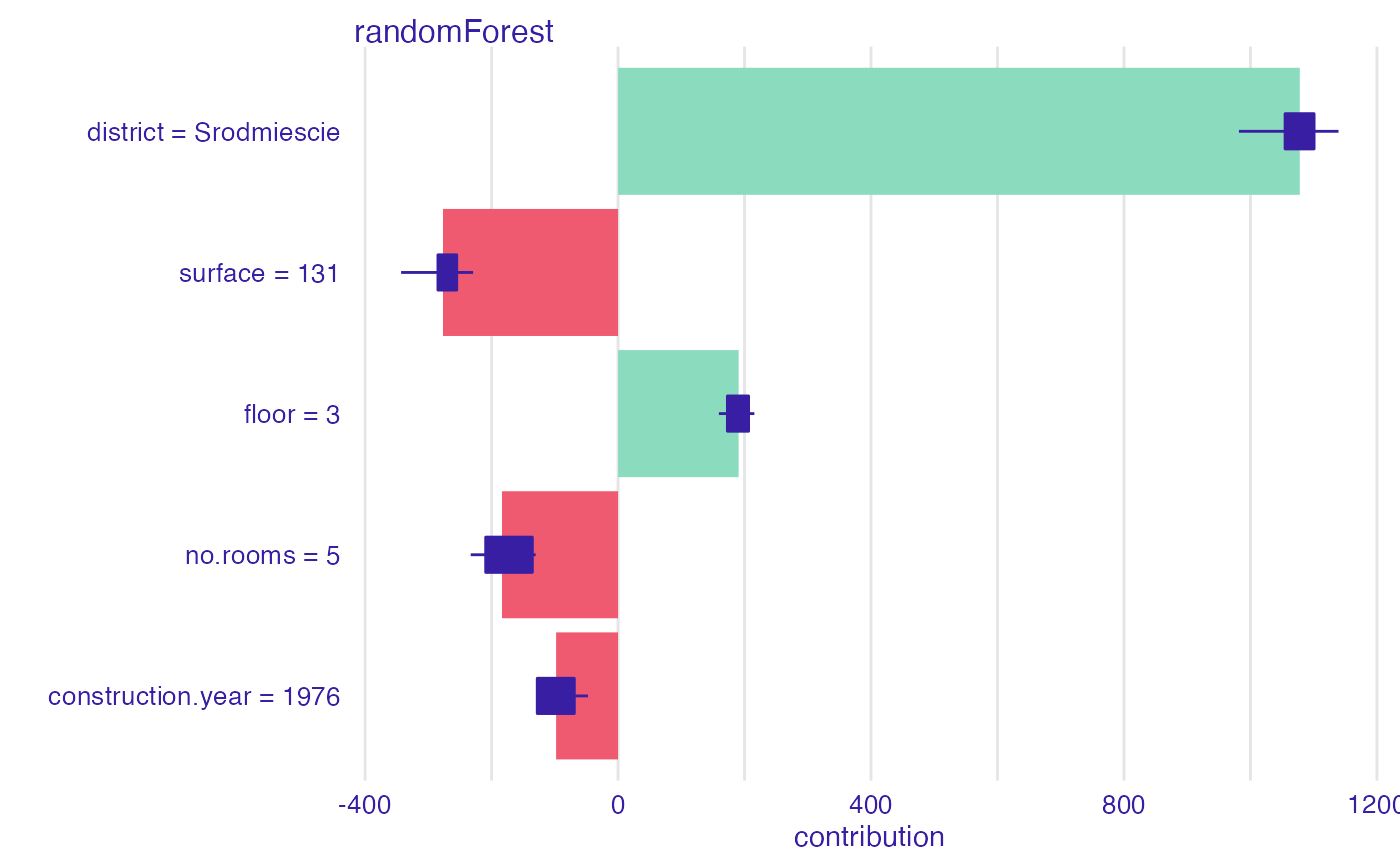
 bd_rf <- break_down_uncertainty(explainer_rf, apartments_test[1,], path = 1:5)
plot(bd_rf)
bd_rf <- break_down_uncertainty(explainer_rf, apartments_test[1,], path = 1:5)
plot(bd_rf)
 bd_rf <- break_down_uncertainty(explainer_rf,
apartments_test[1,],
path = c("floor", "no.rooms", "district",
"construction.year", "surface"))
plot(bd_rf)
bd_rf <- break_down_uncertainty(explainer_rf,
apartments_test[1,],
path = c("floor", "no.rooms", "district",
"construction.year", "surface"))
plot(bd_rf)
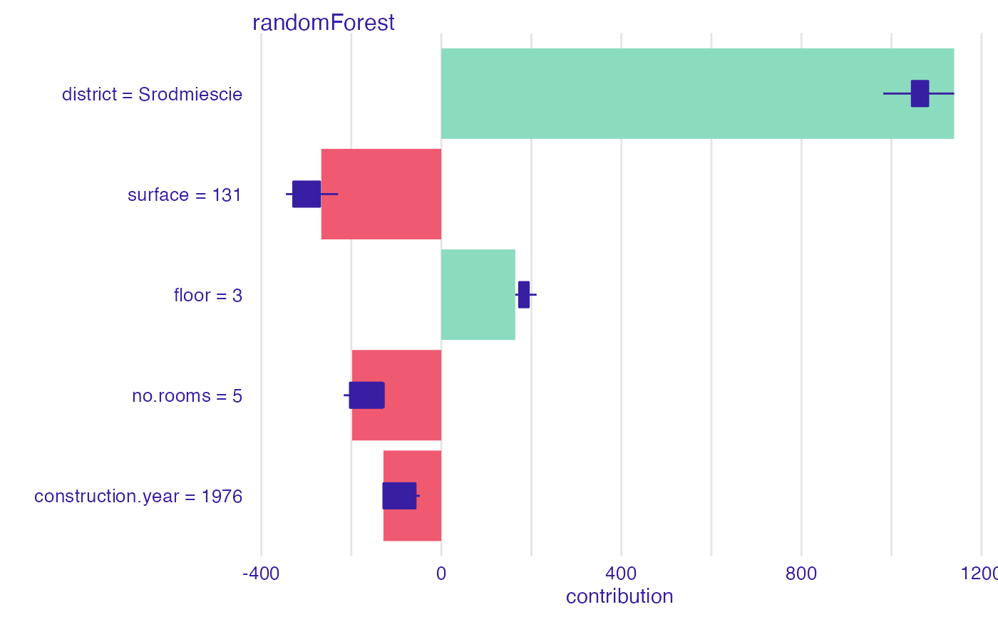
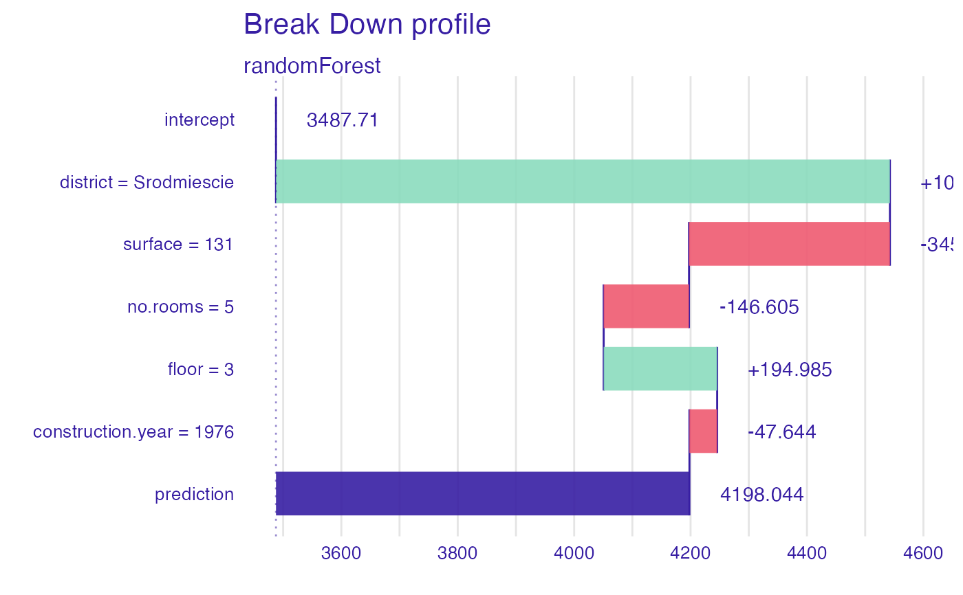
 bd <- break_down(explainer_rf,
apartments_test[1,])
plot(bd)
bd <- break_down(explainer_rf,
apartments_test[1,])
plot(bd)
 s <- shap(explainer_rf,
apartments_test[1,])
plot(s)
s <- shap(explainer_rf,
apartments_test[1,])
plot(s)
 # }
# }