Overall Interaction Strength

Friedman and Popescu's statistic of overall interaction strength per feature, see Details. Use plot() to get a barplot.

h2_overall(object, ...)

# Default S3 method
h2_overall(object, ...)

# S3 method for class 'hstats'
h2_overall(
  object,
  normalize = TRUE,
  squared = TRUE,
  sort = TRUE,
  zero = TRUE,
  ...
)

Arguments

object: Object of class "hstats".
...: Currently unused.
normalize: Should statistics be normalized? Default is TRUE.
squared: Should squared statistics be returned? Default is TRUE.
sort: Should results be sorted? Default is TRUE. (Multi-output is sorted by row means.)
zero: Should rows with all 0 be shown? Default is TRUE.

Value

An object of class "hstats_matrix" containing these elements:

M: Matrix of statistics (one column per prediction dimension), or NULL.
SE: Matrix with standard errors of M, or NULL. Multiply with sqrt(m_rep) to get standard deviations instead. Currently, supported only for perm_importance().
m_rep: The number of repetitions behind standard errors SE, or NULL. Currently, supported only for perm_importance().
statistic: Name of the function that generated the statistic.
description: Description of the statistic.

Details

The logic of Friedman and Popescu (2008) is as follows: If there are no interactions involving feature $x_j$, we can decompose the (centered) prediction function $F$ into the sum of the (centered) partial dependence $F_j$ on $x_j$ and the (centered) partial dependence $F_{\setminus j}$ on all other features $\mathbf{x}_{\setminus j}$, i.e., $$ F(\mathbf{x}) = F_j(x_j) + F_{\setminus j}(\mathbf{x}_{\setminus j}). $$ Correspondingly, Friedman and Popescu's statistic of overall interaction strength of $x_j$ is given by $$ H_j^2 = \frac{\frac{1}{n} \sum_{i = 1}^n\big[F(\mathbf{x}_i) - \hat F_j(x_{ij}) - \hat F_{\setminus j}(\mathbf{x}_{i\setminus j}) \big]^2}{\frac{1}{n} \sum_{i = 1}^n\big[F(\mathbf{x}_i)\big]^2} $$ (check partial_dep() for all definitions).

Remarks:

Partial dependence functions (and $F$) are all centered to (possibly weighted) mean 0.
Partial dependence functions (and $F$) are evaluated over the data distribution. This is different to partial dependence plots, where one uses a fixed grid.
Weighted versions follow by replacing all arithmetic means by corresponding weighted means.
Multivariate predictions can be treated in a component-wise manner.
Due to (typically undesired) extrapolation effects of partial dependence functions, depending on the model, values above 1 may occur.
$H^2_j = 0$ means there are no interactions associated with $x_j$. The higher the value, the more prediction variability comes from interactions with $x_j$.
Since the denominator is the same for all features, the values of the test statistics can be compared across features.

Methods (by class)

h2_overall(default): Default method of overall interaction strength.
h2_overall(hstats): Overall interaction strength from "hstats" object.

References

Friedman, Jerome H., and Bogdan E. Popescu. "Predictive Learning via Rule Ensembles." The Annals of Applied Statistics 2, no. 3 (2008): 916-54.

Examples

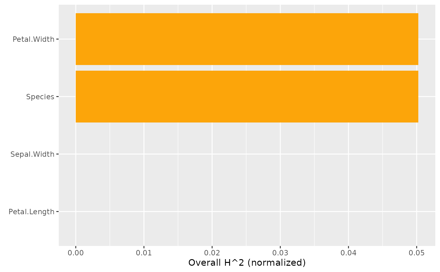
# MODEL 1: Linear regression
fit <- lm(Sepal.Length ~ . + Petal.Width:Species, data = iris)
s <- hstats(fit, X = iris[, -1])
#> 1-way calculations...
#> 
  |                                                                            
  |                                                                      |   0%
  |                                                                            
  |==================                                                    |  25%
  |                                                                            
  |===================================                                   |  50%
  |                                                                            
  |====================================================                  |  75%
  |                                                                            
  |======================================================================| 100%
#> 2-way calculations...
#> 
  |                                                                            
  |                                                                      |   0%
  |                                                                            
  |======================================================================| 100%
h2_overall(s)
#> Overall H^2 (normalized)
#>  Petal.Width      Species  Sepal.Width Petal.Length 
#>    0.0502364    0.0502364    0.0000000    0.0000000 
plot(h2_overall(s))


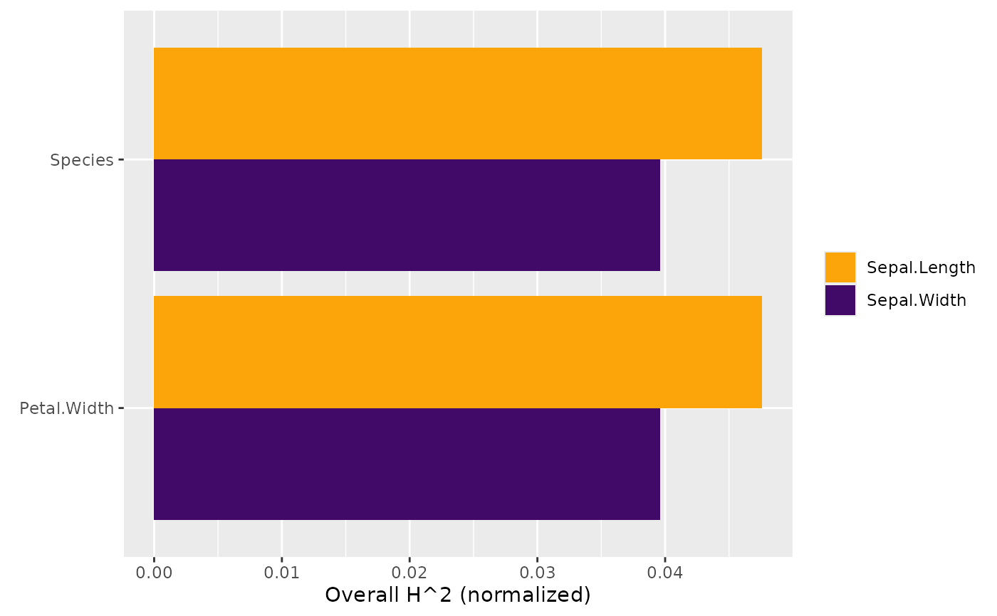
# MODEL 2: Multi-response linear regression
fit <- lm(as.matrix(iris[, 1:2]) ~ Petal.Length + Petal.Width * Species, data = iris)
s <- hstats(fit, X = iris[, 3:5], verbose = FALSE)
plot(h2_overall(s, zero = FALSE))