Three-way Interaction Strength

Friedman and Popescu's statistic of three-way interaction strength, see Details. Use plot() to get a barplot. In hstats(), set threeway_m to a value above 2 to calculate this statistic for all feature triples of the threeway_m features with strongest overall interaction.

h2_threeway(object, ...)

# Default S3 method
h2_threeway(object, ...)

# S3 method for class 'hstats'
h2_threeway(
  object,
  normalize = TRUE,
  squared = TRUE,
  sort = TRUE,
  zero = TRUE,
  ...
)

Arguments

object: Object of class "hstats".
...: Currently unused.
normalize: Should statistics be normalized? Default is TRUE.
squared: Should squared statistics be returned? Default is TRUE.
sort: Should results be sorted? Default is TRUE. (Multi-output is sorted by row means.)
zero: Should rows with all 0 be shown? Default is TRUE.

Value

An object of class "hstats_matrix" containing these elements:

M: Matrix of statistics (one column per prediction dimension), or NULL.
SE: Matrix with standard errors of M, or NULL. Multiply with sqrt(m_rep) to get standard deviations instead. Currently, supported only for perm_importance().
m_rep: The number of repetitions behind standard errors SE, or NULL. Currently, supported only for perm_importance().
statistic: Name of the function that generated the statistic.
description: Description of the statistic.

Details

Friedman and Popescu (2008) describe a test statistic to measure three-way interactions: in case there are no three-way interactions between features $x_j$, $x_k$ and $x_l$, their (centered) three-dimensional partial dependence function $F_{jkl}$ can be decomposed into lower order terms: $$ F_{jkl}(x_j, x_k, x_l) = B_{jkl} - C_{jkl} $$ with $$ B_{jkl} = F_{jk}(x_j, x_k) + F_{jl}(x_j, x_l) + F_{kl}(x_k, x_l) $$ and $$ C_{jkl} = F_j(x_j) + F_k(x_k) + F_l(x_l). $$

The squared and scaled difference between the two sides of the equation leads to the statistic $$ H_{jkl}^2 = \frac{\frac{1}{n} \sum_{i = 1}^n \big[\hat F_{jkl}(x_{ij}, x_{ik}, x_{il}) - B^{(i)}_{jkl} + C^{(i)}_{jkl}\big]^2}{\frac{1}{n} \sum_{i = 1}^n \hat F_{jkl}(x_{ij}, x_{ik}, x_{il})^2}, $$ where $$ B^{(i)}_{jkl} = \hat F_{jk}(x_{ij}, x_{ik}) + \hat F_{jl}(x_{ij}, x_{il}) + \hat F_{kl}(x_{ik}, x_{il}) $$ and $$ C^{(i)}_{jkl} = \hat F_j(x_{ij}) + \hat F_k(x_{ik}) + \hat F_l(x_{il}). $$ Similar remarks as for h2_pairwise() apply.

Methods (by class)

h2_threeway(default): Default pairwise interaction strength.
h2_threeway(hstats): Pairwise interaction strength from "hstats" object.

References

Friedman, Jerome H., and Bogdan E. Popescu. "Predictive Learning via Rule Ensembles." The Annals of Applied Statistics 2, no. 3 (2008): 916-54.

Examples

# MODEL 1: Linear regression
fit <- lm(uptake ~ Type * Treatment * conc, data = CO2)
s <- hstats(fit, X = CO2[, 2:4], threeway_m = 5)
#> 1-way calculations...
#> 
  |                                                                            
  |                                                                      |   0%
  |                                                                            
  |=======================                                               |  33%
  |                                                                            
  |===============================================                       |  67%
  |                                                                            
  |======================================================================| 100%
#> 2-way calculations...
#> 
  |                                                                            
  |                                                                      |   0%
  |                                                                            
  |=======================                                               |  33%
  |                                                                            
  |===============================================                       |  67%
  |                                                                            
  |======================================================================| 100%
#> 3-way calculations...
#> 
  |                                                                            
  |                                                                      |   0%
  |                                                                            
  |======================================================================| 100%
h2_threeway(s)
#> Three-way H^2 (normalized)
#> Type:Treatment:conc 
#>         0.007756484 

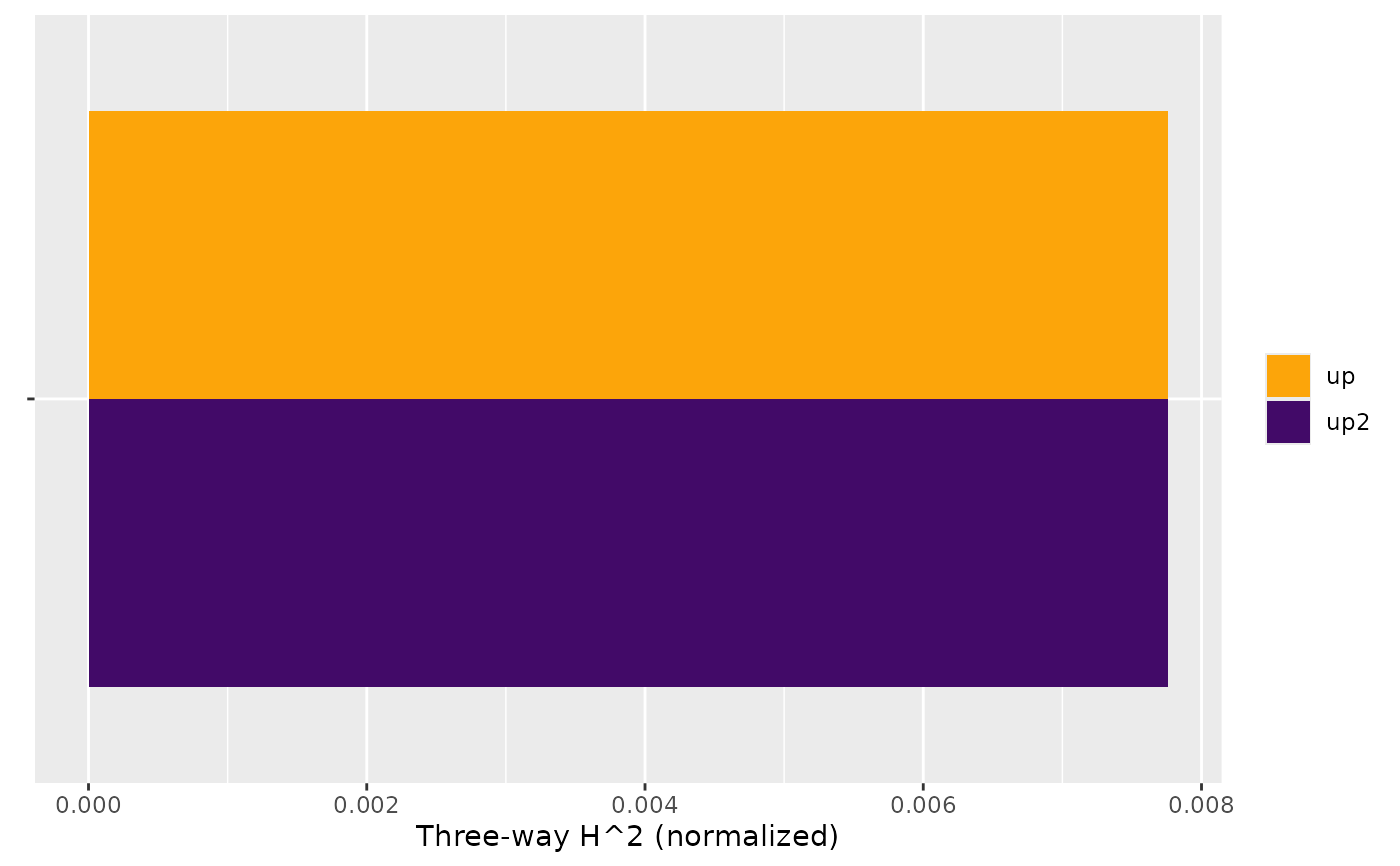
#' MODEL 2: Multivariate output (taking just twice the same response as example)
fit <- lm(cbind(up = uptake, up2 = 2 * uptake) ~ Type * Treatment * conc, data = CO2)
s <- hstats(fit, X = CO2[, 2:4], threeway_m = 5)
#> 1-way calculations...
#> 
  |                                                                            
  |                                                                      |   0%
  |                                                                            
  |=======================                                               |  33%
  |                                                                            
  |===============================================                       |  67%
  |                                                                            
  |======================================================================| 100%
#> 2-way calculations...
#> 
  |                                                                            
  |                                                                      |   0%
  |                                                                            
  |=======================                                               |  33%
  |                                                                            
  |===============================================                       |  67%
  |                                                                            
  |======================================================================| 100%
#> 3-way calculations...
#> 
  |                                                                            
  |                                                                      |   0%
  |                                                                            
  |======================================================================| 100%
h2_threeway(s)
#> Three-way H^2 (normalized)
#>                              up         up2
#> Type:Treatment:conc 0.007756484 0.007756484
h2_threeway(s, normalize = FALSE, squared = FALSE)  # Unnormalized H
#> Three-way H (unnormalized)
#>                            up      up2
#> Type:Treatment:conc 0.8130973 1.626195
plot(h2_threeway(s))