This is the main function of the package. It does the expensive calculations behind the following H-statistics:
Total interaction strength \(H^2\), a statistic measuring the proportion of prediction variability unexplained by main effects of
v, seeh2()for details.Friedman and Popescu's statistic \(H^2_j\) of overall interaction strength per feature, see
h2_overall()for details.Friedman and Popescu's statistic \(H^2_{jk}\) of pairwise interaction strength, see
h2_pairwise()for details.Friedman and Popescu's statistic \(H^2_{jkl}\) of three-way interaction strength, see
h2_threeway()for details. To save time, this statistic is not calculated by default. Setthreeway_mto a value above 2 to get three-way statistics of thethreeway_mvariables with strongest overall interaction.
Furthermore, it allows to calculate an experimental partial dependence based
measure of feature importance, \(\textrm{PDI}_j^2\). It equals the proportion of
prediction variability unexplained by other features, see pd_importance()
for details. This statistic is not shown by summary() or plot().
Instead of using summary(), interaction statistics can also be obtained via the
more flexible functions h2(), h2_overall(), h2_pairwise(), and
h2_threeway().
hstats(object, ...)

# Default S3 method
hstats(
  object,
  X,
  v = NULL,
  pred_fun = stats::predict,
  pairwise_m = 5L,
  threeway_m = 0L,
  approx = FALSE,
  grid_size = 50L,
  n_max = 500L,
  eps = 1e-10,
  w = NULL,
  verbose = TRUE,
  ...
)

# S3 method for class 'ranger'
hstats(
  object,
  X,
  v = NULL,
  pred_fun = NULL,
  pairwise_m = 5L,
  threeway_m = 0L,
  approx = FALSE,
  grid_size = 50L,
  n_max = 500L,
  eps = 1e-10,
  w = NULL,
  verbose = TRUE,
  survival = c("chf", "prob"),
  ...
)

# S3 method for class 'explainer'
hstats(
  object,
  X = object[["data"]],
  v = NULL,
  pred_fun = object[["predict_function"]],
  pairwise_m = 5L,
  threeway_m = 0L,
  approx = FALSE,
  grid_size = 50L,
  n_max = 500L,
  eps = 1e-10,
  w = object[["weights"]],
  verbose = TRUE,
  ...
)
Arguments
- object
Fitted model object.
- ...
Additional arguments passed to
pred_fun(object, X, ...), for instancetype = "response"in aglm()model, orreshape = TRUEin a multiclass XGBoost model.- X
A data.frame or matrix serving as background dataset.
- v
Vector of feature names. The default (
NULL) will use all column names ofXexcept the column name of the optional case weightw(if specified as name).- pred_fun
Prediction function of the form
function(object, X, ...), providing \(K \ge 1\) predictions per row. Its first argument represents the modelobject, its second argument a data structure likeX. Additional arguments (such astype = "response"in a GLM, orreshape = TRUEin a multiclass XGBoost model) can be passed via.... The default,stats::predict(), will work in most cases.- pairwise_m
Number of features for which pairwise statistics are to be calculated. The features are selected based on Friedman and Popescu's overall interaction strength \(H^2_j\). Set to to 0 to avoid pairwise calculations. For multivariate predictions, the union of the
pairwise_mcolumn-wise strongest variable names is taken. This can lead to very long run-times.- threeway_m
Like
pairwise_m, but controls the feature count for three-way interactions. Cannot be larger thanpairwise_m. To save computation time, the default is 0.- approx
Should quantile approximation be applied to dense numeric features? The default is
FALSE. Setting this option toTRUEbrings a massive speed-up for one-way calculations. It can, e.g., be used when the number of features is very large.- grid_size
Integer controlling the number of quantile midpoints used to approximate dense numerics. The quantile midpoints are calculated after subampling via
n_max. Only relevant ifapprox = TRUE.- n_max
If
Xhas more thann_maxrows, a random sample ofn_maxrows is selected fromX. In this case, set a random seed for reproducibility.- eps
Threshold below which numerator values are set to 0. Default is 1e-10.
- w
Optional vector of case weights. Can also be a column name of
X.- verbose
Should a progress bar be shown? The default is
TRUE.- survival
Should cumulative hazards ("chf", default) or survival probabilities ("prob") per time be predicted? Only in
ranger()survival models.
Value
An object of class "hstats" containing these elements:
X: InputX(sampled ton_maxrows, after optional quantile approximation).w: Case weight vectorw(sampled ton_maxvalues), orNULL.v: Vector of column names inXfor which overall H statistics have been calculated.f: Matrix with (centered) predictions \(F\).mean_f2: (Weighted) column means off. Used to normalize \(H^2\) and \(H^2_j\).F_j: List of matrices, each representing (centered) partial dependence functions \(F_j\).F_not_j: List of matrices with (centered) partial dependence functions \(F_{\setminus j}\) of other features.K: Number of columns of prediction matrix.pred_names: Column names of prediction matrix.pairwise_m: Like inputpairwise_m, but capped atlength(v).threeway_m: Like inputthreeway_m, but capped at the smaller oflength(v)andpairwise_m.eps: Like inputeps.pd_importance: List with numerator and denominator of \(\textrm{PDI}_j\).h2: List with numerator and denominator of \(H^2\).h2_overall: List with numerator and denominator of \(H^2_j\).v_pairwise: Subset ofvwith largest \(H^2_j\) used for pairwise calculations. Only if pairwise calculations have been done.combs2: Named list of variable pairs for which pairwise partial dependence functions are available. Only if pairwise calculations have been done.F_jk: List of matrices, each representing (centered) bivariate partial dependence functions \(F_{jk}\). Only if pairwise calculations have been done.h2_pairwise: List with numerator and denominator of \(H^2_{jk}\). Only if pairwise calculations have been done.v_threeway: Subset ofvwith largesth2_overall()used for three-way calculations. Only if three-way calculations have been done.combs3: Named list of variable triples for which three-way partial dependence functions are available. Only if three-way calculations have been done.F_jkl: List of matrices, each representing (centered) three-way partial dependence functions \(F_{jkl}\). Only if three-way calculations have been done.h2_threeway: List with numerator and denominator of \(H^2_{jkl}\). Only if three-way calculations have been done.
Methods (by class)
hstats(default): Default hstats method.hstats(ranger): Method for "ranger" models.hstats(explainer): Method for DALEX "explainer".
References
Friedman, Jerome H., and Bogdan E. Popescu. "Predictive Learning via Rule Ensembles." The Annals of Applied Statistics 2, no. 3 (2008): 916-54.
See also
h2(), h2_overall(), h2_pairwise(), h2_threeway(),
and pd_importance() for specific statistics calculated from the resulting object.
Examples
# MODEL 1: Linear regression
fit <- lm(Sepal.Length ~ . + Petal.Width:Species, data = iris)
s <- hstats(fit, X = iris[, -1])
#> 1-way calculations...
#>
|
| | 0%
|
|================== | 25%
|
|=================================== | 50%
|
|==================================================== | 75%
|
|======================================================================| 100%
#> 2-way calculations...
#>
|
| | 0%
|
|======================================================================| 100%
s
#> 'hstats' object. Use plot() or summary() for details.
#>
#> H^2 (normalized)
#> [1] 0.0502364
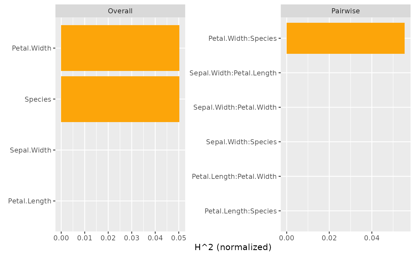
plot(s)
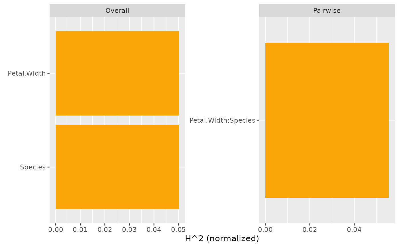
 plot(s, zero = FALSE) # Drop 0
 summary(s)
#> *H^2 (normalized)
#> [1] 0.0502364
#>
#> *Largest Overall H^2 (normalized)
#> Petal.Width Species Sepal.Width Petal.Length
#> 0.0502364 0.0502364 0.0000000 0.0000000
#>
#> *Largest Pairwise H^2 (normalized)
#> [,1]
#> Petal.Width:Species 0.05546172
#> Sepal.Width:Petal.Length 0.00000000
#> Sepal.Width:Petal.Width 0.00000000
#>
# Absolute pairwise interaction strengths
h2_pairwise(s, normalize = FALSE, squared = FALSE, zero = FALSE)
#> Pairwise H (unnormalized)
#> Petal.Width:Species
#> 0.1726312
# MODEL 2: Multi-response linear regression
fit <- lm(as.matrix(iris[, 1:2]) ~ Petal.Length + Petal.Width * Species, data = iris)
s <- hstats(fit, X = iris[, 3:5], verbose = FALSE)
plot(s)
summary(s)
#> *H^2 (normalized)
#> [1] 0.0502364
#>
#> *Largest Overall H^2 (normalized)
#> Petal.Width Species Sepal.Width Petal.Length
#> 0.0502364 0.0502364 0.0000000 0.0000000
#>
#> *Largest Pairwise H^2 (normalized)
#> [,1]
#> Petal.Width:Species 0.05546172
#> Sepal.Width:Petal.Length 0.00000000
#> Sepal.Width:Petal.Width 0.00000000
#>
# Absolute pairwise interaction strengths
h2_pairwise(s, normalize = FALSE, squared = FALSE, zero = FALSE)
#> Pairwise H (unnormalized)
#> Petal.Width:Species
#> 0.1726312
# MODEL 2: Multi-response linear regression
fit <- lm(as.matrix(iris[, 1:2]) ~ Petal.Length + Petal.Width * Species, data = iris)
s <- hstats(fit, X = iris[, 3:5], verbose = FALSE)
plot(s)
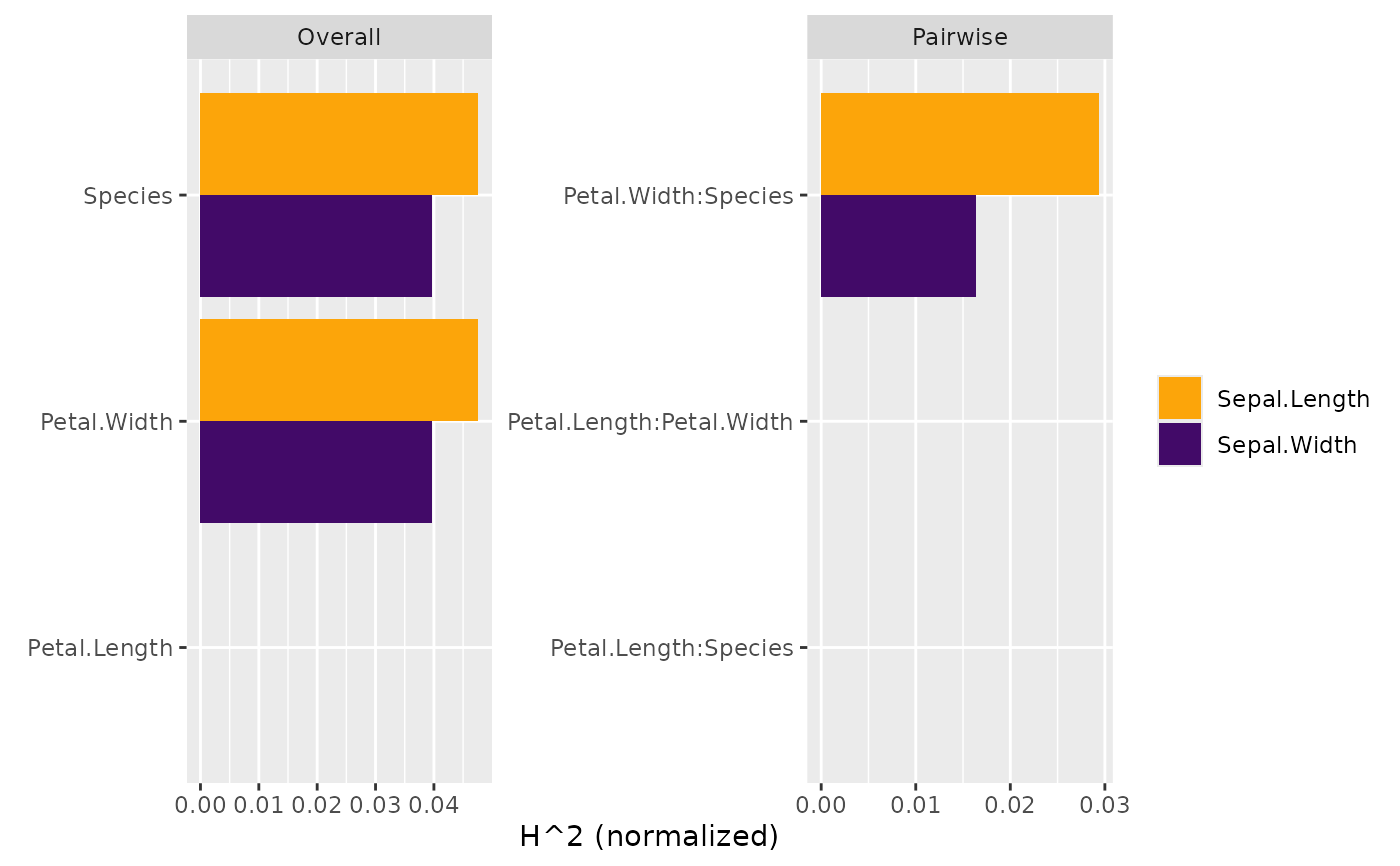 summary(s)
#> *H^2 (normalized)
#> Sepal.Length Sepal.Width
#> 0.04758952 0.03963575
#>
#> *Largest Overall H^2 (normalized)
#> Sepal.Length Sepal.Width
#> Species 0.04758952 0.03963575
#> Petal.Width 0.04758952 0.03963575
#> Petal.Length 0.00000000 0.00000000
#>
#> *Largest Pairwise H^2 (normalized)
#> Sepal.Length Sepal.Width
#> Petal.Width:Species 0.02937378 0.01637166
#> Petal.Length:Petal.Width 0.00000000 0.00000000
#> Petal.Length:Species 0.00000000 0.00000000
#>
# MODEL 3: Gamma GLM with log link
fit <- glm(Sepal.Length ~ ., data = iris, family = Gamma(link = log))
# No interactions for additive features, at least on link scale
s <- hstats(fit, X = iris[, -1], verbose = FALSE)
summary(s)
#> *H^2 (normalized)
#> [1] 0
#>
#> *Largest Overall H^2 (normalized)
#> Sepal.Width Petal.Length Petal.Width Species
#> 0 0 0 0
#>
#> *Largest Pairwise H^2 (normalized)
#> [,1]
#> Sepal.Width:Petal.Length 0
#> Sepal.Width:Petal.Width 0
#> Sepal.Width:Species 0
#>
# On original scale, we have interactions everywhere.
# To see three-way interactions, we set threeway_m to a value above 2.
s <- hstats(fit, X = iris[, -1], type = "response", threeway_m = 5)
#> 1-way calculations...
#>
|
| | 0%
|
|================== | 25%
|
|=================================== | 50%
|
|==================================================== | 75%
|
|======================================================================| 100%
#> 2-way calculations...
#>
|
| | 0%
|
|============ | 17%
|
|======================= | 33%
|
|=================================== | 50%
|
|=============================================== | 67%
|
|========================================================== | 83%
|
|======================================================================| 100%
#> 3-way calculations...
#>
|
| | 0%
|
|================== | 25%
|
|=================================== | 50%
|
|==================================================== | 75%
|
|======================================================================| 100%
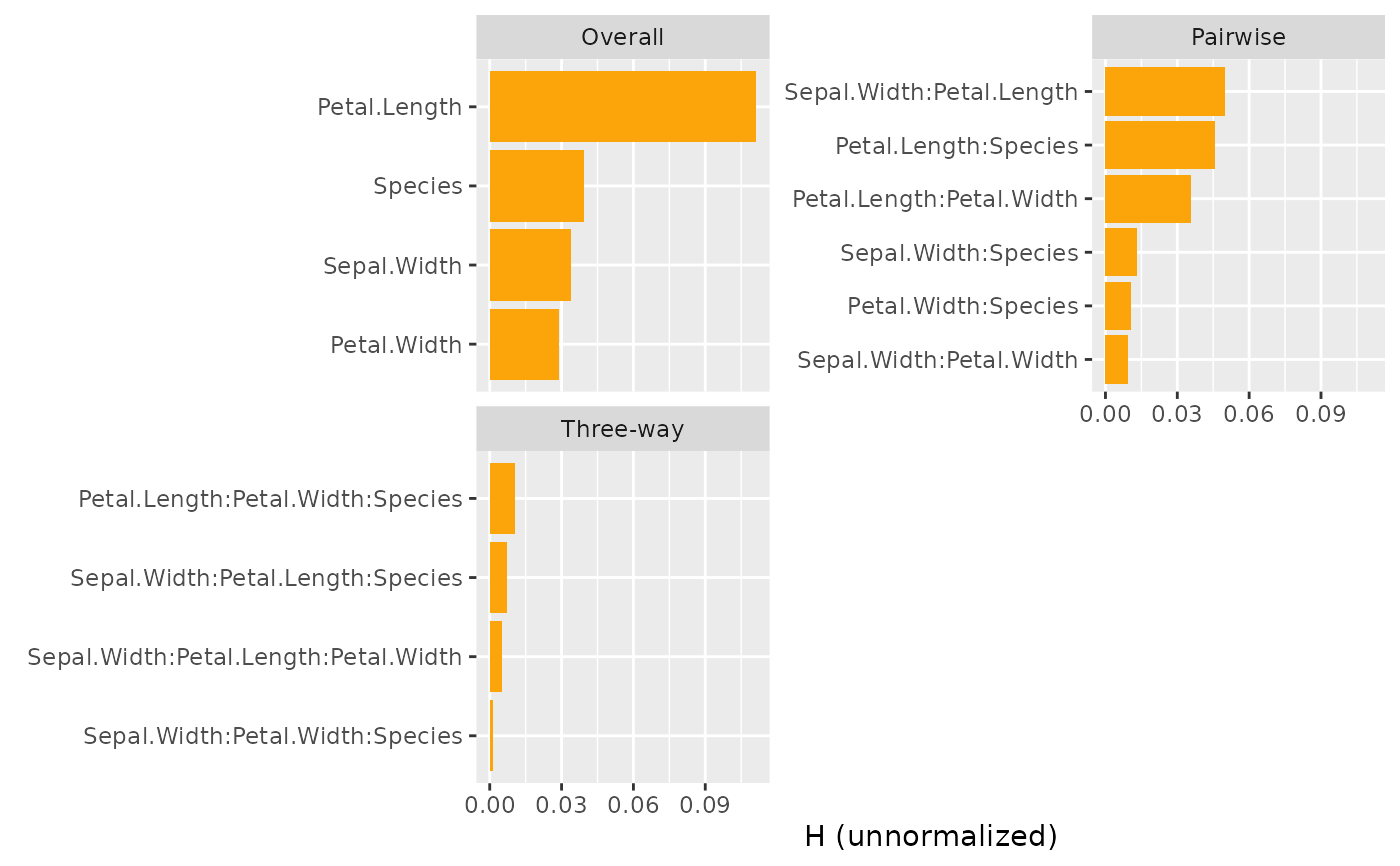
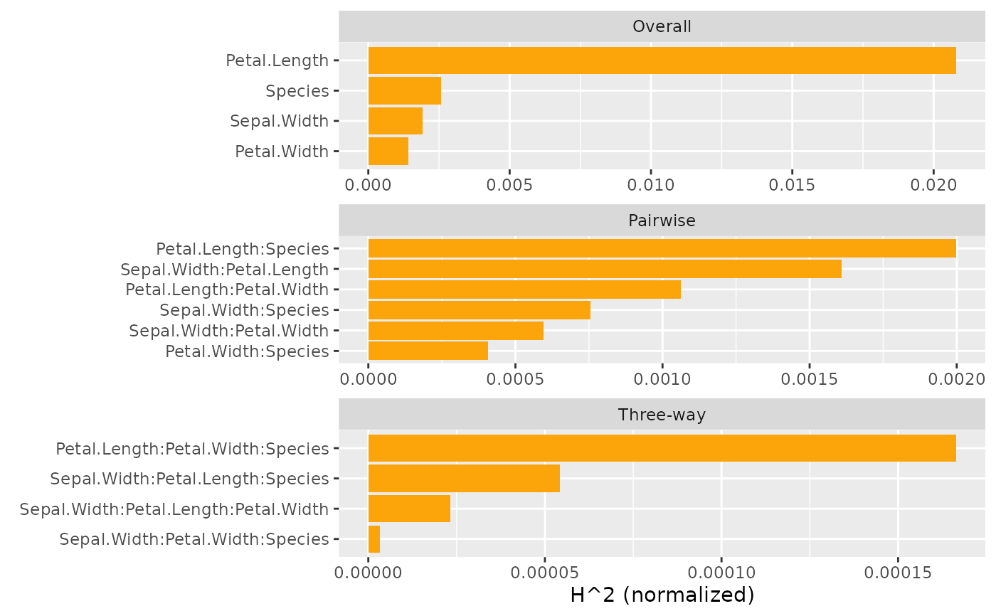
plot(s, ncol = 1) # All three types use different denominators
summary(s)
#> *H^2 (normalized)
#> Sepal.Length Sepal.Width
#> 0.04758952 0.03963575
#>
#> *Largest Overall H^2 (normalized)
#> Sepal.Length Sepal.Width
#> Species 0.04758952 0.03963575
#> Petal.Width 0.04758952 0.03963575
#> Petal.Length 0.00000000 0.00000000
#>
#> *Largest Pairwise H^2 (normalized)
#> Sepal.Length Sepal.Width
#> Petal.Width:Species 0.02937378 0.01637166
#> Petal.Length:Petal.Width 0.00000000 0.00000000
#> Petal.Length:Species 0.00000000 0.00000000
#>
# MODEL 3: Gamma GLM with log link
fit <- glm(Sepal.Length ~ ., data = iris, family = Gamma(link = log))
# No interactions for additive features, at least on link scale
s <- hstats(fit, X = iris[, -1], verbose = FALSE)
summary(s)
#> *H^2 (normalized)
#> [1] 0
#>
#> *Largest Overall H^2 (normalized)
#> Sepal.Width Petal.Length Petal.Width Species
#> 0 0 0 0
#>
#> *Largest Pairwise H^2 (normalized)
#> [,1]
#> Sepal.Width:Petal.Length 0
#> Sepal.Width:Petal.Width 0
#> Sepal.Width:Species 0
#>
# On original scale, we have interactions everywhere.
# To see three-way interactions, we set threeway_m to a value above 2.
s <- hstats(fit, X = iris[, -1], type = "response", threeway_m = 5)
#> 1-way calculations...
#>
|
| | 0%
|
|================== | 25%
|
|=================================== | 50%
|
|==================================================== | 75%
|
|======================================================================| 100%
#> 2-way calculations...
#>
|
| | 0%
|
|============ | 17%
|
|======================= | 33%
|
|=================================== | 50%
|
|=============================================== | 67%
|
|========================================================== | 83%
|
|======================================================================| 100%
#> 3-way calculations...
#>
|
| | 0%
|
|================== | 25%
|
|=================================== | 50%
|
|==================================================== | 75%
|
|======================================================================| 100%
plot(s, ncol = 1) # All three types use different denominators
 # All statistics on same scale (of predictions)
plot(s, squared = FALSE, normalize = FALSE, facet_scale = "free_y")
# All statistics on same scale (of predictions)
plot(s, squared = FALSE, normalize = FALSE, facet_scale = "free_y")