Estimates the partial dependence function of feature(s) v over a
grid of values. Both multivariate and multivariable situations are supported.
The resulting object can be plotted via plot().
partial_dep(object, ...)

# Default S3 method
partial_dep(
  object,
  v,
  X,
  pred_fun = stats::predict,
  BY = NULL,
  by_size = 4L,
  grid = NULL,
  grid_size = 49L,
  trim = c(0.01, 0.99),
  strategy = c("uniform", "quantile"),
  na.rm = TRUE,
  n_max = 1000L,
  w = NULL,
  ...
)

# S3 method for class 'ranger'
partial_dep(
  object,
  v,
  X,
  pred_fun = NULL,
  BY = NULL,
  by_size = 4L,
  grid = NULL,
  grid_size = 49L,
  trim = c(0.01, 0.99),
  strategy = c("uniform", "quantile"),
  na.rm = TRUE,
  n_max = 1000L,
  w = NULL,
  survival = c("chf", "prob"),
  ...
)

# S3 method for class 'explainer'
partial_dep(
  object,
  v,
  X = object[["data"]],
  pred_fun = object[["predict_function"]],
  BY = NULL,
  by_size = 4L,
  grid = NULL,
  grid_size = 49L,
  trim = c(0.01, 0.99),
  strategy = c("uniform", "quantile"),
  na.rm = TRUE,
  n_max = 1000L,
  w = object[["weights"]],
  ...
)
Arguments
- object
Fitted model object.
- ...
Additional arguments passed to
pred_fun(object, X, ...), for instancetype = "response"in aglm()model, orreshape = TRUEin a multiclass XGBoost model.- v
One or more column names over which you want to calculate the partial dependence.
- X
A data.frame or matrix serving as background dataset.
- pred_fun
Prediction function of the form
function(object, X, ...), providing \(K \ge 1\) predictions per row. Its first argument represents the modelobject, its second argument a data structure likeX. Additional arguments (such astype = "response"in a GLM, orreshape = TRUEin a multiclass XGBoost model) can be passed via.... The default,stats::predict(), will work in most cases.- BY
Optional grouping vector or column name. The partial dependence function is calculated per
BYgroup. EachBYgroup uses the same evaluation grid to improve assessment of (non-)additivity. NumericBYvariables with more thanby_sizedisjoint values will be binned intoby_sizequantile groups of similar size. To improve robustness, subsampling ofXis done within group. This only applies toBYgroups with more thann_maxrows.- by_size
Numeric
BYvariables with more thanby_sizeunique values will be binned into quantile groups. Only relevant ifBYis notNULL.- grid
Evaluation grid. A vector (if
length(v) == 1L), or a matrix/data.frame otherwise. IfNULL, calculated viamultivariate_grid().- grid_size
Controls the approximate grid size. If
xhas p columns, then each (non-discrete) column will be reduced to about the p-th root ofgrid_sizevalues.- trim
The default
c(0.01, 0.99)means that values outside the 1% and 99% quantiles of non-discrete numeric columns are removed before calculation of grid values. Set to0:1for no trimming.- strategy
How to find grid values of non-discrete numeric columns? Either "uniform" or "quantile", see description of
univariate_grid().- na.rm
Should missing values be dropped from the grid? Default is
TRUE.- n_max
If
Xhas more thann_maxrows, a random sample ofn_maxrows is selected fromX. In this case, set a random seed for reproducibility.- w
Optional vector of case weights. Can also be a column name of
X.- survival
Should cumulative hazards ("chf", default) or survival probabilities ("prob") per time be predicted? Only in
ranger()survival models.
Value
An object of class "partial_dep" containing these elements:
data: data.frame containing the partial dependencies.v: Same as inputv.K: Number of columns of prediction matrix.pred_names: Column names of prediction matrix.by_name: Column name of grouping variable (orNULL).
Methods (by class)
partial_dep(default): Default method.partial_dep(ranger): Method for "ranger" models.partial_dep(explainer): Method for DALEX "explainer".
Partial Dependence Functions
Let \(F: R^p \to R\) denote the prediction function that maps the \(p\)-dimensional feature vector \(\mathbf{x} = (x_1, \dots, x_p)\) to its prediction. Furthermore, let $$ F_s(\mathbf{x}_s) = E_{\mathbf{x}_{\setminus s}}(F(\mathbf{x}_s, \mathbf{x}_{\setminus s})) $$ be the partial dependence function of \(F\) on the feature subset \(\mathbf{x}_s\), where \(s \subseteq \{1, \dots, p\}\), as introduced in Friedman (2001). Here, the expectation runs over the joint marginal distribution of features \(\mathbf{x}_{\setminus s}\) not in \(\mathbf{x}_s\).
Given data, \(F_s(\mathbf{x}_s)\) can be estimated by the empirical partial dependence function
$$ \hat F_s(\mathbf{x}_s) = \frac{1}{n} \sum_{i = 1}^n F(\mathbf{x}_s, \mathbf{x}_{i\setminus s}), $$ where \(\mathbf{x}_{i\setminus s}\) \(i = 1, \dots, n\), are the observed values of \(\mathbf{x}_{\setminus s}\).
A partial dependence plot (PDP) plots the values of \(\hat F_s(\mathbf{x}_s)\) over a grid of evaluation points \(\mathbf{x}_s\).
References
Friedman, Jerome H. "Greedy Function Approximation: A Gradient Boosting Machine." Annals of Statistics 29, no. 5 (2001): 1189-1232.
Examples
# MODEL 1: Linear regression
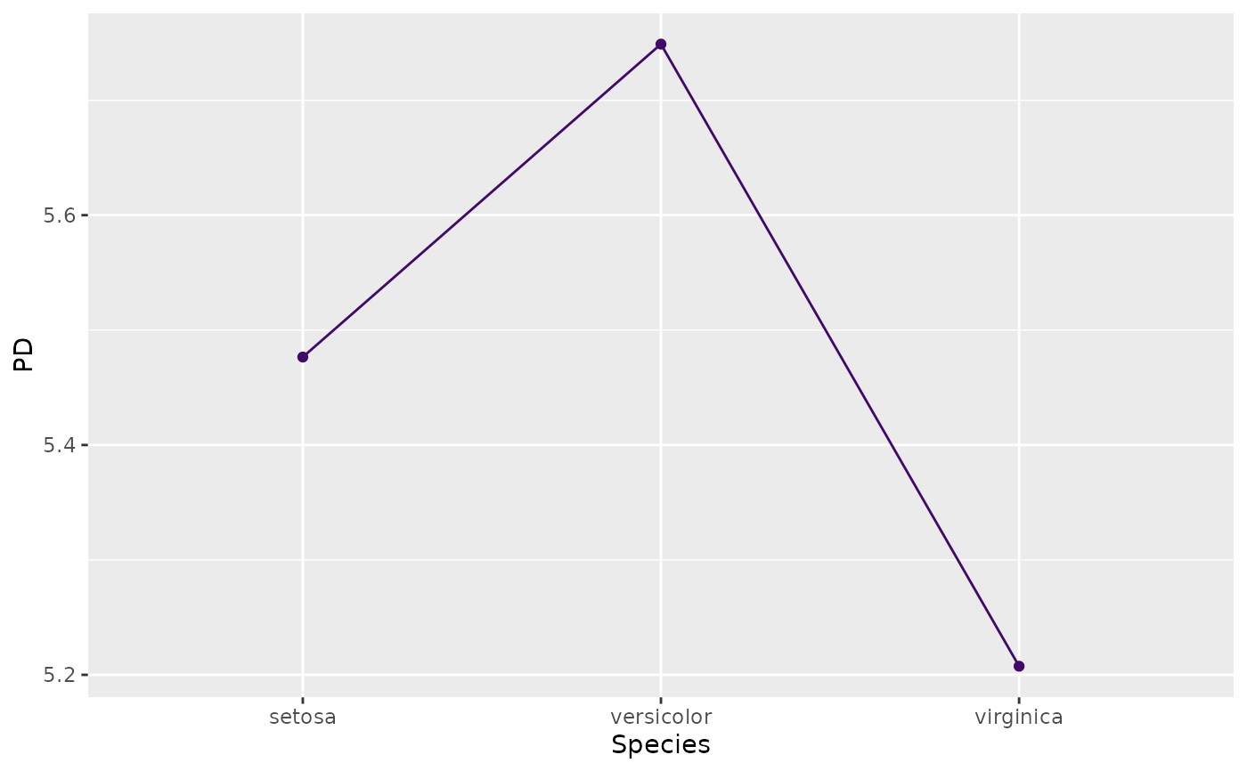
fit <- lm(Sepal.Length ~ . + Species * Petal.Length, data = iris)
(pd <- partial_dep(fit, v = "Species", X = iris))
#> Partial dependence object (3 rows). Extract via $data. Top rows:
#>
#> Species y
#> 1 setosa 5.476540
#> 2 versicolor 5.748857
#> 3 virginica 5.207491
plot(pd)
 if (FALSE) { # \dontrun{
# Stratified by BY variable (numerics are automatically binned)
pd <- partial_dep(fit, v = "Species", X = iris, BY = "Petal.Length")
plot(pd)
# Multivariable input
v <- c("Species", "Petal.Length")
pd <- partial_dep(fit, v = v, X = iris, grid_size = 100L)
plot(pd, rotate_x = TRUE)
plot(pd, d2_geom = "line") # often better to read
# With grouping
pd <- partial_dep(fit, v = v, X = iris, grid_size = 100L, BY = "Petal.Width")
plot(pd, rotate_x = TRUE)
plot(pd, rotate_x = TRUE, d2_geom = "line")
plot(pd, rotate_x = TRUE, d2_geom = "line", swap_dim = TRUE)
# MODEL 2: Multi-response linear regression
fit <- lm(as.matrix(iris[, 1:2]) ~ Petal.Length + Petal.Width * Species, data = iris)
pd <- partial_dep(fit, v = "Petal.Width", X = iris, BY = "Species")
plot(pd, show_points = FALSE)
pd <- partial_dep(fit, v = c("Species", "Petal.Width"), X = iris)
plot(pd, rotate_x = TRUE)
plot(pd, d2_geom = "line", rotate_x = TRUE)
plot(pd, d2_geom = "line", rotate_x = TRUE, swap_dim = TRUE)
# Multivariate, multivariable, and BY (no plot available)
pd <- partial_dep(
fit, v = c("Petal.Width", "Petal.Length"), X = iris, BY = "Species"
)
pd
} # }
# MODEL 3: Gamma GLM -> pass options to predict() via ...
fit <- glm(Sepal.Length ~ ., data = iris, family = Gamma(link = log))
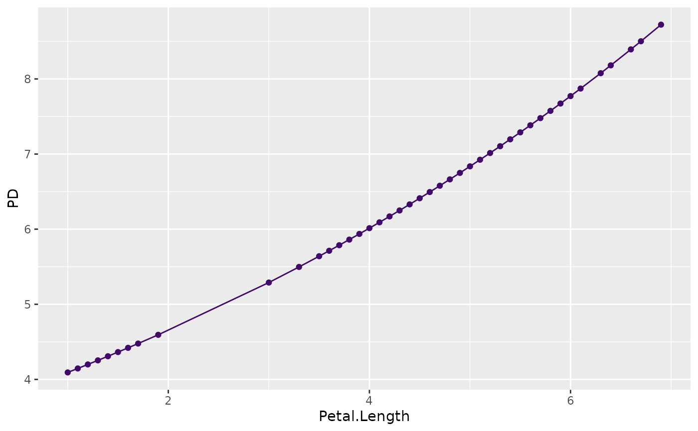
plot(partial_dep(fit, v = "Petal.Length", X = iris), show_points = FALSE)
if (FALSE) { # \dontrun{
# Stratified by BY variable (numerics are automatically binned)
pd <- partial_dep(fit, v = "Species", X = iris, BY = "Petal.Length")
plot(pd)
# Multivariable input
v <- c("Species", "Petal.Length")
pd <- partial_dep(fit, v = v, X = iris, grid_size = 100L)
plot(pd, rotate_x = TRUE)
plot(pd, d2_geom = "line") # often better to read
# With grouping
pd <- partial_dep(fit, v = v, X = iris, grid_size = 100L, BY = "Petal.Width")
plot(pd, rotate_x = TRUE)
plot(pd, rotate_x = TRUE, d2_geom = "line")
plot(pd, rotate_x = TRUE, d2_geom = "line", swap_dim = TRUE)
# MODEL 2: Multi-response linear regression
fit <- lm(as.matrix(iris[, 1:2]) ~ Petal.Length + Petal.Width * Species, data = iris)
pd <- partial_dep(fit, v = "Petal.Width", X = iris, BY = "Species")
plot(pd, show_points = FALSE)
pd <- partial_dep(fit, v = c("Species", "Petal.Width"), X = iris)
plot(pd, rotate_x = TRUE)
plot(pd, d2_geom = "line", rotate_x = TRUE)
plot(pd, d2_geom = "line", rotate_x = TRUE, swap_dim = TRUE)
# Multivariate, multivariable, and BY (no plot available)
pd <- partial_dep(
fit, v = c("Petal.Width", "Petal.Length"), X = iris, BY = "Species"
)
pd
} # }
# MODEL 3: Gamma GLM -> pass options to predict() via ...
fit <- glm(Sepal.Length ~ ., data = iris, family = Gamma(link = log))
plot(partial_dep(fit, v = "Petal.Length", X = iris), show_points = FALSE)
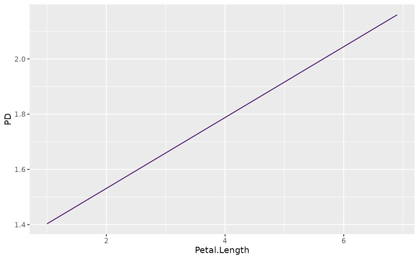 plot(partial_dep(fit, v = "Petal.Length", X = iris, type = "response"))