Plot Dataset Level Model Diagnostics
# S3 method for model_diagnostics
plot(x, ..., variable = "y_hat", yvariable = "residuals", smooth = TRUE)
Arguments
- x
a data.frame to be explained, preprocessed by the
model_diagnosticsfunction- ...
other object to be included to the plot
- variable
character - name of the variable on OX axis to be explained, by default
y_hat- yvariable
character - name of the variable on OY axis, by default
residuals- smooth
logical shall the smooth line be added
Value
an object of the class model_diagnostics_explainer.
Examples
apartments_lm_model <- lm(m2.price ~ ., data = apartments)
explainer_lm <- explain(apartments_lm_model,
data = apartments,
y = apartments$m2.price)
#> Preparation of a new explainer is initiated
#> -> model label : lm ( default )
#> -> data : 1000 rows 6 cols
#> -> target variable : 1000 values
#> -> predict function : yhat.lm will be used ( default )
#> -> predicted values : No value for predict function target column. ( default )
#> -> model_info : package stats , ver. 4.2.3 , task regression ( default )
#> -> predicted values : numerical, min = 1781.848 , mean = 3487.019 , max = 6176.032
#> -> residual function : difference between y and yhat ( default )
#> -> residuals : numerical, min = -247.4728 , mean = 2.093656e-14 , max = 469.0023
#> A new explainer has been created!
diag_lm <- model_diagnostics(explainer_lm)
diag_lm
#> m2.price construction.year surface floor
#> Min. :1607 Min. :1920 Min. : 20.00 Min. : 1.000
#> 1st Qu.:2857 1st Qu.:1943 1st Qu.: 53.00 1st Qu.: 3.000
#> Median :3386 Median :1965 Median : 85.50 Median : 6.000
#> Mean :3487 Mean :1965 Mean : 85.59 Mean : 5.623
#> 3rd Qu.:4018 3rd Qu.:1988 3rd Qu.:118.00 3rd Qu.: 8.000
#> Max. :6595 Max. :2010 Max. :150.00 Max. :10.000
#>
#> no.rooms district y y_hat
#> Min. :1.00 Mokotow :107 Min. :1607 Min. :1782
#> 1st Qu.:2.00 Wola :106 1st Qu.:2857 1st Qu.:2879
#> Median :3.00 Ursus :105 Median :3386 Median :3374
#> Mean :3.36 Ursynow :103 Mean :3487 Mean :3487
#> 3rd Qu.:4.00 Srodmiescie:100 3rd Qu.:4018 3rd Qu.:3932
#> Max. :6.00 Bemowo : 98 Max. :6595 Max. :6176
#> (Other) :381
#> residuals abs_residuals label ids
#> Min. :-247.5 Min. :134.9 Length:1000 Min. : 1.0
#> 1st Qu.:-202.8 1st Qu.:180.3 Class :character 1st Qu.: 250.8
#> Median :-172.8 Median :212.4 Mode :character Median : 500.5
#> Mean : 0.0 Mean :260.0 Mean : 500.5
#> 3rd Qu.: 381.4 3rd Qu.:381.4 3rd Qu.: 750.2
#> Max. : 469.0 Max. :469.0 Max. :1000.0
#>
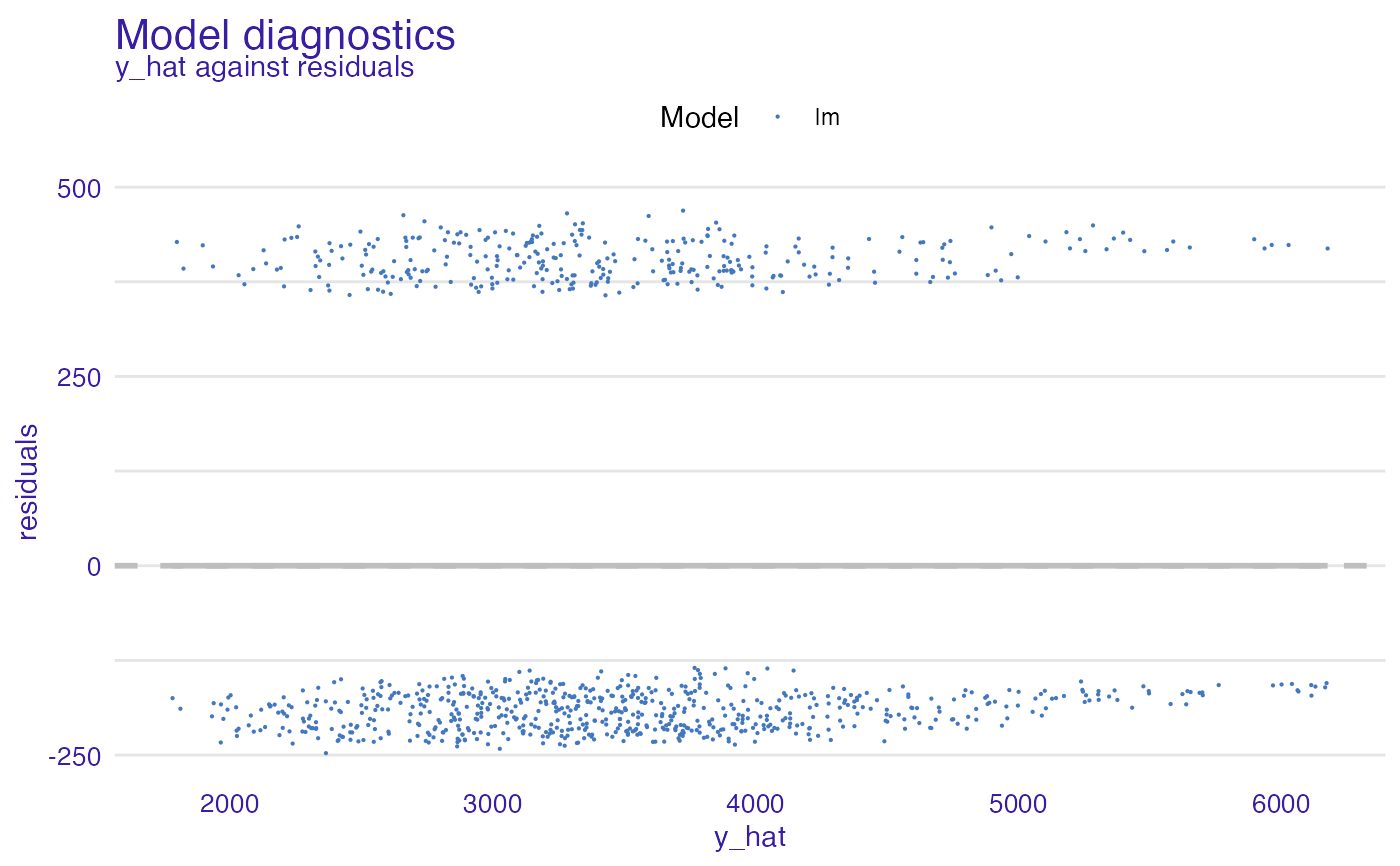
plot(diag_lm)
#> `geom_smooth()` using method = 'gam' and formula = 'y ~ s(x, bs = "cs")'
 # \donttest{
library("ranger")
apartments_ranger_model <- ranger(m2.price ~ ., data = apartments)
explainer_ranger <- explain(apartments_ranger_model,
data = apartments,
y = apartments$m2.price)
#> Preparation of a new explainer is initiated
#> -> model label : ranger ( default )
#> -> data : 1000 rows 6 cols
#> -> target variable : 1000 values
#> -> predict function : yhat.ranger will be used ( default )
#> -> predicted values : No value for predict function target column. ( default )
#> -> model_info : package ranger , ver. 0.14.1 , task regression ( default )
#> -> predicted values : numerical, min = 1866.438 , mean = 3488.478 , max = 6164.809
#> -> residual function : difference between y and yhat ( default )
#> -> residuals : numerical, min = -423.0415 , mean = -1.459128 , max = 591.9183
#> A new explainer has been created!
diag_ranger <- model_diagnostics(explainer_ranger)
diag_ranger
#> m2.price construction.year surface floor
#> Min. :1607 Min. :1920 Min. : 20.00 Min. : 1.000
#> 1st Qu.:2857 1st Qu.:1943 1st Qu.: 53.00 1st Qu.: 3.000
#> Median :3386 Median :1965 Median : 85.50 Median : 6.000
#> Mean :3487 Mean :1965 Mean : 85.59 Mean : 5.623
#> 3rd Qu.:4018 3rd Qu.:1988 3rd Qu.:118.00 3rd Qu.: 8.000
#> Max. :6595 Max. :2010 Max. :150.00 Max. :10.000
#>
#> no.rooms district y y_hat
#> Min. :1.00 Mokotow :107 Min. :1607 Min. :1866
#> 1st Qu.:2.00 Wola :106 1st Qu.:2857 1st Qu.:2941
#> Median :3.00 Ursus :105 Median :3386 Median :3413
#> Mean :3.36 Ursynow :103 Mean :3487 Mean :3488
#> 3rd Qu.:4.00 Srodmiescie:100 3rd Qu.:4018 3rd Qu.:3952
#> Max. :6.00 Bemowo : 98 Max. :6595 Max. :6165
#> (Other) :381
#> residuals abs_residuals label ids
#> Min. :-423.041 Min. : 0.197 Length:1000 Min. : 1.0
#> 1st Qu.: -91.739 1st Qu.: 38.809 Class :character 1st Qu.: 250.8
#> Median : -28.641 Median : 81.443 Mode :character Median : 500.5
#> Mean : -1.459 Mean :107.439 Mean : 500.5
#> 3rd Qu.: 63.584 3rd Qu.:147.811 3rd Qu.: 750.2
#> Max. : 591.918 Max. :591.918 Max. :1000.0
#>
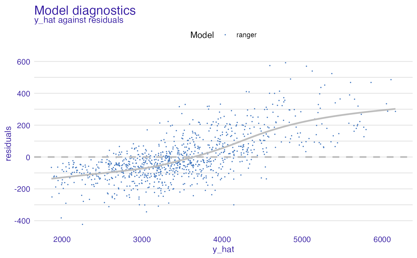
plot(diag_ranger)
#> `geom_smooth()` using method = 'gam' and formula = 'y ~ s(x, bs = "cs")'
# \donttest{
library("ranger")
apartments_ranger_model <- ranger(m2.price ~ ., data = apartments)
explainer_ranger <- explain(apartments_ranger_model,
data = apartments,
y = apartments$m2.price)
#> Preparation of a new explainer is initiated
#> -> model label : ranger ( default )
#> -> data : 1000 rows 6 cols
#> -> target variable : 1000 values
#> -> predict function : yhat.ranger will be used ( default )
#> -> predicted values : No value for predict function target column. ( default )
#> -> model_info : package ranger , ver. 0.14.1 , task regression ( default )
#> -> predicted values : numerical, min = 1866.438 , mean = 3488.478 , max = 6164.809
#> -> residual function : difference between y and yhat ( default )
#> -> residuals : numerical, min = -423.0415 , mean = -1.459128 , max = 591.9183
#> A new explainer has been created!
diag_ranger <- model_diagnostics(explainer_ranger)
diag_ranger
#> m2.price construction.year surface floor
#> Min. :1607 Min. :1920 Min. : 20.00 Min. : 1.000
#> 1st Qu.:2857 1st Qu.:1943 1st Qu.: 53.00 1st Qu.: 3.000
#> Median :3386 Median :1965 Median : 85.50 Median : 6.000
#> Mean :3487 Mean :1965 Mean : 85.59 Mean : 5.623
#> 3rd Qu.:4018 3rd Qu.:1988 3rd Qu.:118.00 3rd Qu.: 8.000
#> Max. :6595 Max. :2010 Max. :150.00 Max. :10.000
#>
#> no.rooms district y y_hat
#> Min. :1.00 Mokotow :107 Min. :1607 Min. :1866
#> 1st Qu.:2.00 Wola :106 1st Qu.:2857 1st Qu.:2941
#> Median :3.00 Ursus :105 Median :3386 Median :3413
#> Mean :3.36 Ursynow :103 Mean :3487 Mean :3488
#> 3rd Qu.:4.00 Srodmiescie:100 3rd Qu.:4018 3rd Qu.:3952
#> Max. :6.00 Bemowo : 98 Max. :6595 Max. :6165
#> (Other) :381
#> residuals abs_residuals label ids
#> Min. :-423.041 Min. : 0.197 Length:1000 Min. : 1.0
#> 1st Qu.: -91.739 1st Qu.: 38.809 Class :character 1st Qu.: 250.8
#> Median : -28.641 Median : 81.443 Mode :character Median : 500.5
#> Mean : -1.459 Mean :107.439 Mean : 500.5
#> 3rd Qu.: 63.584 3rd Qu.:147.811 3rd Qu.: 750.2
#> Max. : 591.918 Max. :591.918 Max. :1000.0
#>
plot(diag_ranger)
#> `geom_smooth()` using method = 'gam' and formula = 'y ~ s(x, bs = "cs")'
 plot(diag_ranger, diag_lm)
#> `geom_smooth()` using method = 'gam' and formula = 'y ~ s(x, bs = "cs")'
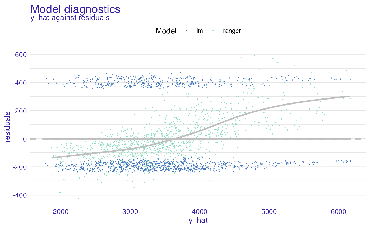
plot(diag_ranger, diag_lm)
#> `geom_smooth()` using method = 'gam' and formula = 'y ~ s(x, bs = "cs")'
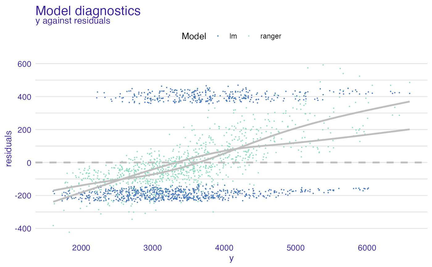
 plot(diag_ranger, diag_lm, variable = "y")
#> `geom_smooth()` using method = 'gam' and formula = 'y ~ s(x, bs = "cs")'
plot(diag_ranger, diag_lm, variable = "y")
#> `geom_smooth()` using method = 'gam' and formula = 'y ~ s(x, bs = "cs")'
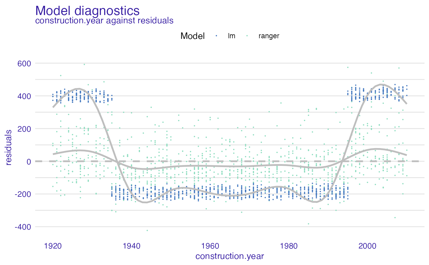
 plot(diag_ranger, diag_lm, variable = "construction.year")
#> `geom_smooth()` using method = 'gam' and formula = 'y ~ s(x, bs = "cs")'
plot(diag_ranger, diag_lm, variable = "construction.year")
#> `geom_smooth()` using method = 'gam' and formula = 'y ~ s(x, bs = "cs")'
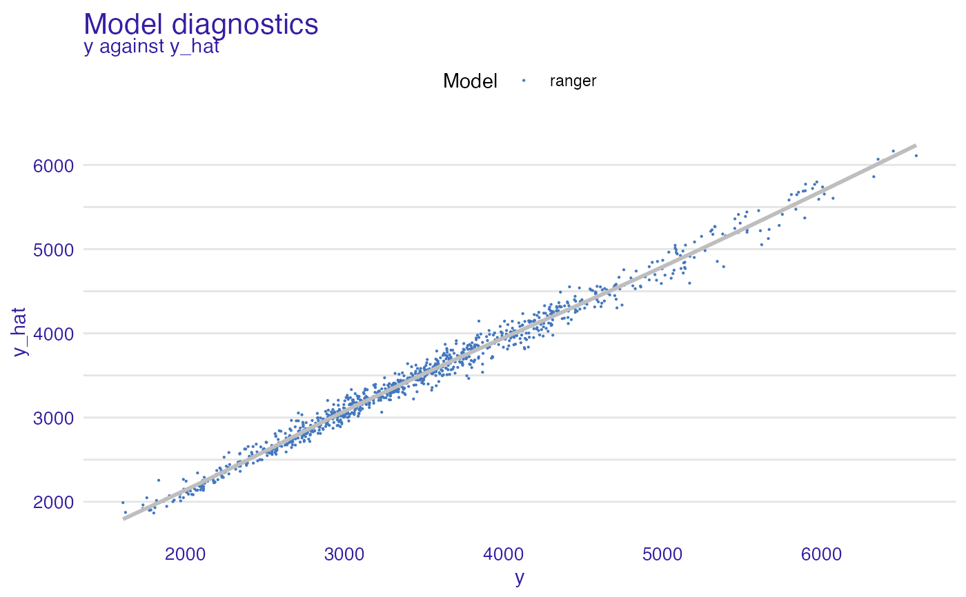
 plot(diag_ranger, variable = "y", yvariable = "y_hat")
#> `geom_smooth()` using method = 'gam' and formula = 'y ~ s(x, bs = "cs")'
plot(diag_ranger, variable = "y", yvariable = "y_hat")
#> `geom_smooth()` using method = 'gam' and formula = 'y ~ s(x, bs = "cs")'
 # }
# }