Methods and xspliner environment
Krystian Igras
2019-10-05
methods.RmdPredict
As xspliner final model is GLM, predict method is just wrapper of stats::predict.glm function. Let’s see it on the below example:
library(xspliner)
library(randomForest)
library(magrittr)

rf_iris <- randomForest(Petal.Width ~  Sepal.Length + Petal.Length + Species, data = iris)
model_xs <- xspline(Petal.Width ~
  Sepal.Length +
  xs(Petal.Length, effect = list(grid.resolution = 100), transition = list(bs = "cr")) +
  xf(Species, transition = list(stat = "loglikelihood", value = -300)),
  model = rf_iris)
newdata <- data.frame(
  Sepal.Length = 10,
  Petal.Length = 2,
  Species = factor("virginica", levels = levels(iris$Species)))
predict(model_xs, newdata = newdata)
## 1
## -0.2733431Print method works similarly to the summary. In case of passing just the model, standard print.glm is used.
##
## Call:  stats::glm(formula = Petal.Width ~ Sepal.Length + xs(Petal.Length) +
##     xf(Species), family = family, data = data)
##
## Coefficients:
##                    (Intercept)                    Sepal.Length
##                       -2.05021                        -0.01101
##               xs(Petal.Length)  xf(Species)versicolorvirginica
##                        3.11587                        -0.52469
##
## Degrees of Freedom: 149 Total (i.e. Null);  146 Residual
## Null Deviance:       86.57
## Residual Deviance: 5.15  AIC: -70.05
Predictor based print
Summary method allows you to check details about transformation of specific variable.
Standard usage print(xspliner_object, variable_name)
Quantitative variable
When predictor is the quantitative variable its transition is based on GAM model. For this case print uses standard print.gam method.
##
## Family: gaussian
## Link function: identity
##
## Formula:
## yhat ~ s(Petal.Length, bs = "cr")
##
## Estimated degrees of freedom:
## 8.81  total = 9.81
##
## GCV score: 0.001295152
Qualitative variable
In case of qualitative predictor, standard print.factorMerger method is used.
## Family: gaussian Factor Merger.
##
## Factor levels were merged in the following order:
##
##      groupA       groupB                     model   pvalVsFull   pvalVsPrevious
## ---  -----------  --------------------  ----------  -----------  ---------------
## 0                                        -257.9975            1                1
## 1    versicolor   virginica              -273.2059            0                0
## 2    setosa       versicolorvirginica    -352.6976            0                0
Plot
You can see all details in graphics
Transition
Transition method allows you to extract objects used during building transition of variables. There are three possible object types that can be extracted.
Extracting effect
Each transition is built on top of the black box response data. For example the default response for quantitative variables is PDP - for qualitative ones ICE.
In order to extract the effect use transition method with type parameter equals to data
##   Petal.Length      yhat
## 1     1.000000 0.7466766
## 2     1.059596 0.7466766
## 3     1.119192 0.7466766
## 4     1.178788 0.7499946
## 5     1.238384 0.7514118
## 6 1.297980 0.7542732## Species yhat yhat.id
## 1 setosa 0.2463188 1
## 2 versicolor 0.7119859 1
## 3 virginica 0.8650061 1
## 4 setosa 0.2210225 2
## 5 versicolor 0.7027318 2
## 6 virginica 0.8558598 2Extracting transition model
After we built transition basing on continuity of variable specific model is created. In case of quantitative predictor we build GAM model in order to get spline approximation of effect. In case of qualitative predictor we build factorMerger object and get optimal factor division on that.
To extract the model, use transition method with type = "base":
##
## Family: gaussian
## Link function: identity
##
## Formula:
## yhat ~ s(Petal.Length, bs = "cr")
##
## Estimated degrees of freedom:
## 8.81  total = 9.81
##
## GCV score: 0.001295152## Family: gaussian Factor Merger.
##
## Factor levels were merged in the following order:
##
## groupA groupB model pvalVsFull pvalVsPrevious
## --- ----------- -------------------- ---------- ----------- ---------------
## 0 -257.9975 1 1
## 1 versicolor virginica -273.2059 0 0
## 2 setosa versicolorvirginica -352.6976 0 0Extracting transition function
The final result of building transition is transformation function, that is used in the final GLM model estimation.
To extract the function just use transition method with type = "function".
petal_length_xs <- transition(model_xs, predictor = "Petal.Length", type = "function")
x <- seq(1, 7, length.out = 50)
plot(x, petal_length_xs(x))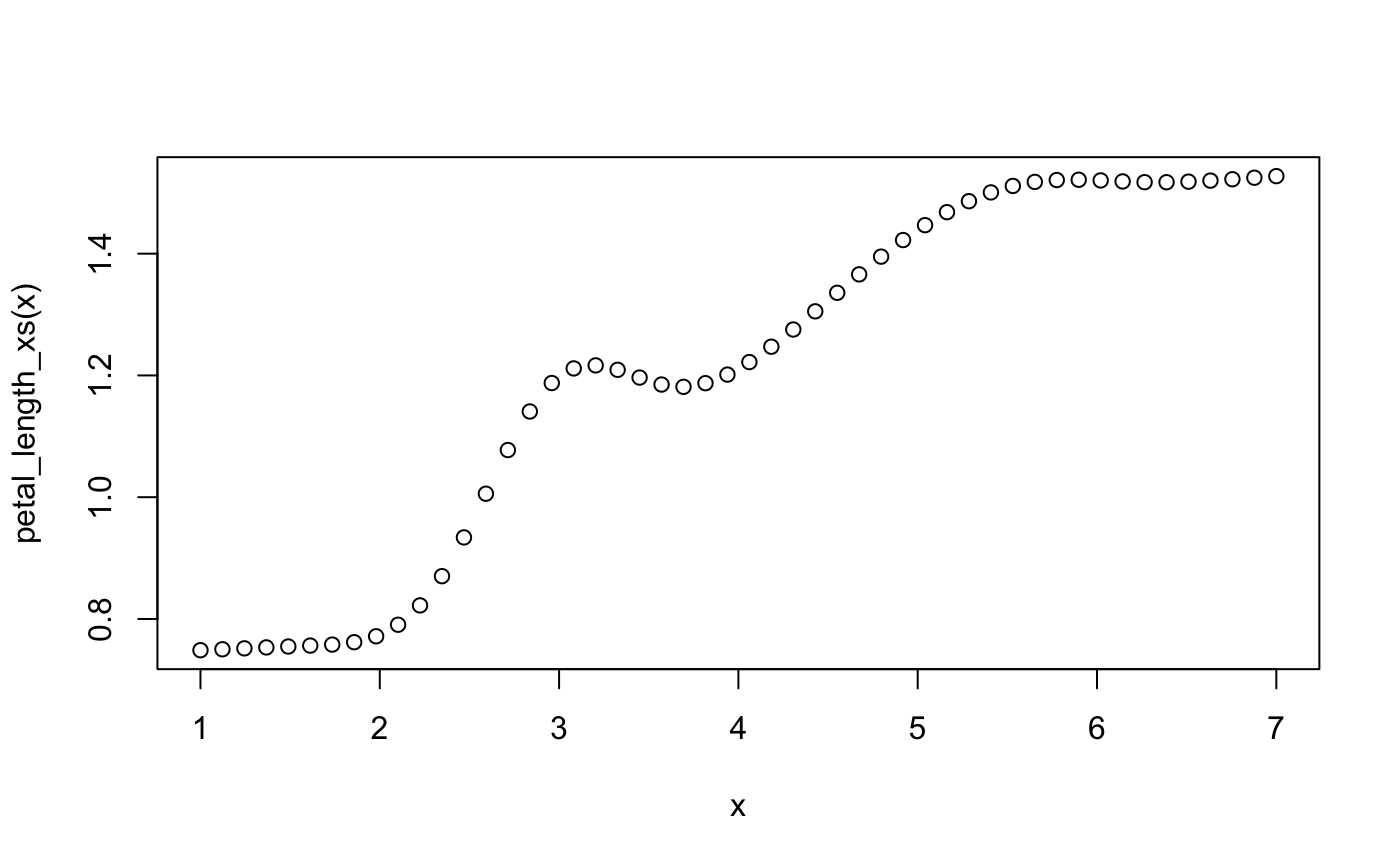
species_xf <- transition(model_xs, predictor = "Species", type = "function")
species_xf(c("setosa", "versicolor", "virginica"))
## [1] setosa versicolorvirginica versicolorvirginica
## Levels: setosa versicolorvirginicaSummary
Summary method allows you to check the basic model details. See below what possibilities the method to xspliner model offers.
GLM summary
Standard summary method is just wrapper for summary::glm. In order to use this just type:
##
## Call:
## stats::glm(formula = Petal.Width ~ Sepal.Length + xs(Petal.Length) +
##     xf(Species), family = family, data = data)
##
## Deviance Residuals:
##      Min        1Q    Median        3Q       Max
## -0.67996  -0.07974  -0.01344   0.10639   0.49730
##
## Coefficients:
##                                Estimate Std. Error t value Pr(>|t|)
## (Intercept)                    -2.05021    0.14181 -14.458  < 2e-16 ***
## Sepal.Length                   -0.01101    0.03623  -0.304    0.762
## xs(Petal.Length)                3.11587    0.21528  14.474  < 2e-16 ***
## xf(Species)versicolorvirginica -0.52469    0.11510  -4.559 1.08e-05 ***
## ---
## Signif. codes:  0 '***' 0.001 '**' 0.01 '*' 0.05 '.' 0.1 ' ' 1
##
## (Dispersion parameter for gaussian family taken to be 0.03527647)
##
##     Null deviance: 86.5699  on 149  degrees of freedom
## Residual deviance:  5.1504  on 146  degrees of freedom
## AIC: -70.054
##
## Number of Fisher Scoring iterations: 2
Predictor based summary
Summary method allows you to check details about transformation of specific variable.
Standard usage summary(xspliner_object, variable_name)
Quantitative variable
When predictor is quantitative variable its transition is based on GAM model. For this case summary displays summary of that model.
##
## Family: gaussian
## Link function: identity
##
## Formula:
## yhat ~ s(Petal.Length, bs = "cr")
##
## Parametric coefficients:
##             Estimate Std. Error t value Pr(>|t|)
## (Intercept) 1.204452   0.003418   352.4   <2e-16 ***
## ---
## Signif. codes:  0 '***' 0.001 '**' 0.01 '*' 0.05 '.' 0.1 ' ' 1
##
## Approximate significance of smooth terms:
##                   edf Ref.df     F p-value
## s(Petal.Length) 8.808  8.989 771.6  <2e-16 ***
## ---
## Signif. codes:  0 '***' 0.001 '**' 0.01 '*' 0.05 '.' 0.1 ' ' 1
##
## R-sq.(adj) =  0.986   Deviance explained = 98.7%
## GCV = 0.0012952  Scale est. = 0.0011681  n = 100
Qualitative variable
In case of qualitative predictor, the method displays data.frame storing information how factors were merged during the transition.
##         orig                pred
## 1     setosa              setosa
## 2 versicolor versicolorvirginica
## 3  virginica versicolorvirginica
Surrogate vs Black Box comparison
Providing model parameter instead of predictor, the summary displays a few statistics that compares original model with surrogate one. All statistics definitions are included in summary.xspline documentation.
Here we show one example for classification model.
For this example we use ISLR::Default data and build svm model as black box. The model aims to predict default variable, indicating whether the customer defaulted on their debt.
## Warning: package 'e1071' was built under R version 3.5.2set.seed(1)
data <- ISLR::Default
default.svm <- svm(default ~ ., data = data, probability = TRUE)
default.xs <- xspline(default ~ student + xs(balance) + xs(income), model = default.svm)In order to check the summary, we need to specify prediction functions for each model. In this case predictions are probabilities of success:
prob_svm <- function(object, newdata) attr(predict(object, newdata = newdata, probability = TRUE), "probabilities")[, 2]
prob_xs <- function(object, newdata) predict(object, newdata = newdata, type = "response")
Almost each summary statistic compares models basing on some data.
In this case we’re going to compare models on training data providing:
-
newdataparameter as training data -
modelparameter with black box model -
prediction_funsas a list of prediction functions (for surrogate and original model respectively)
## Models comparison
##   1 - Max prediction normed-diff:  0.5268109
##   R^2:  0.9185403
## Setting levels: control = No, case = Yes
## Setting levels: control = No, case = Yes## 1 - Max ROC diff: 0.8712113
## 1 - Mean ROC diff: 0.9506292Another set of statistics is generated for prediction functions that return response levels.
response_svm <- function(object, newdata) predict(object, newdata = newdata)
response_xs <- function(object, newdata) {
  y_levels <- levels(newdata[[environment(object)$response]])
  factor(y_levels[(predict.glm(object, newdata = newdata, type = "link") > 0) + 1], levels = y_levels)
}
And similarly to previous example:
summary(default.xs, model = default.svm, newdata = data, prediction_funs = list(response_xs, response_svm))## Models comparison
## Mean predictions similarity: 0.9966
## ACC Black Box: 0.9719
## ACC Surrogate: 0.9729