Example of local variable importance

In this vignette, we present a local variable importance measure based on Ceteris Paribus profiles for random forest regression model.

1 Dataset

We work on Apartments dataset from DALEX package.

#>   m2.price construction.year surface floor no.rooms    district
#> 1     5897              1953      25     3        1 Srodmiescie
#> 2     1818              1992     143     9        5     Bielany
#> 3     3643              1937      56     1        2       Praga
#> 4     3517              1995      93     7        3      Ochota
#> 5     3013              1992     144     6        5     Mokotow
#> 6     5795              1926      61     6        2 Srodmiescie

2 Random forest regression model

Now, we define a random forest regression model and use explain from DALEX.

library("randomForest")
apartments_rf_model <- randomForest(m2.price ~ construction.year + surface + floor +
                                      no.rooms, data = apartments)
explainer_rf <- explain(apartments_rf_model,
                        data = apartmentsTest[,2:5], y = apartmentsTest$m2.price)
#> Preparation of a new explainer is initiated
#>   -> model label       :  randomForest  ( [33m default [39m )
#>   -> data              :  9000  rows  4  cols 
#>   -> target variable   :  9000  values 
#>   -> predict function  :  yhat.randomForest  will be used ( [33m default [39m )
#>   -> predicted values  :  numerical, min =  2093.577 , mean =  3514.544 , max =  5329.173  
#>   -> model_info        :  package randomForest , ver. 4.6.14 , task regression ( [33m default [39m ) 
#>   -> residual function :  difference between y and yhat ( [33m default [39m )
#>   -> residuals         :  numerical, min =  -1193.497 , mean =  -3.020797 , max =  2140.187  
#>  [32m A new explainer has been created! [39m

3 New observation

We need to specify an observation. Let consider a new apartment with the following attributes. Moreover, we calculate predict value for this new observation.

new_apartment <- data.frame(construction.year = 1998, surface = 88, floor = 2L, no.rooms = 3)
predict(apartments_rf_model, new_apartment)
#>        1 
#> 3882.594

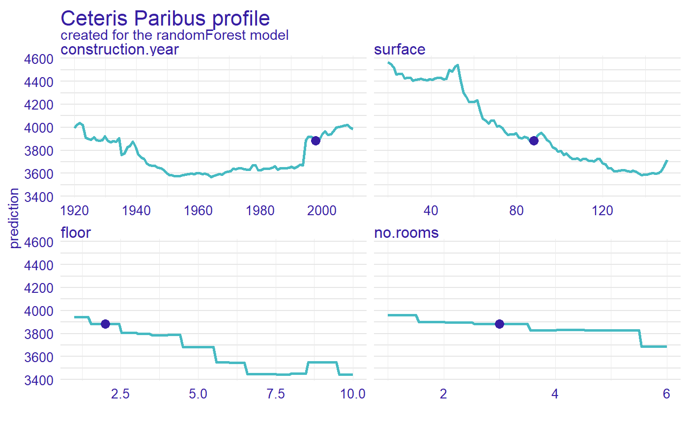
4 Calculate Ceteris Paribus profiles

Let see the Ceteris Paribus Plots calculated with DALEX::predict_profile() function. The CP also can be calculated with DALEX::individual_profile() or ingredients::ceteris_paribus().

library("ingredients")
profiles <- predict_profile(explainer_rf, new_apartment)
plot(profiles) + show_observations(profiles)

5 Calculate measure of local variable importance

Now, we calculated a measure of local variable importance via oscillation based on Ceteris Paribus profiles. We use variant with all parameters equals to TRUE.

library("vivo")
measure <- local_variable_importance(profiles, apartments[,2:5],
            absolute_deviation = TRUE, point = TRUE, density = TRUE)

plot(measure)

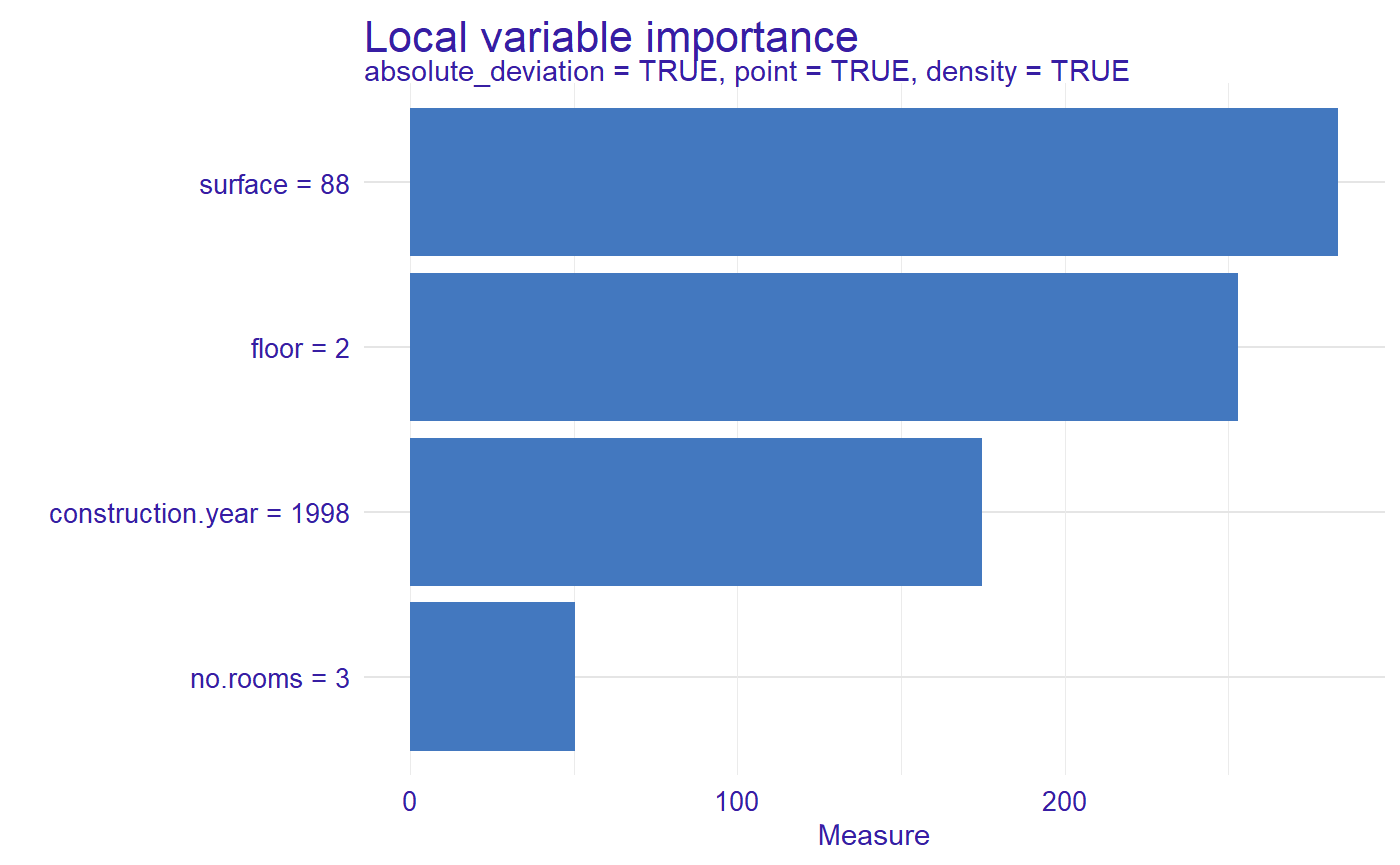
For the new observation the most important variable is surface, then floor, construction.year and no.rooms.

6 Comparison of two or more methods of calculating the importance of variables

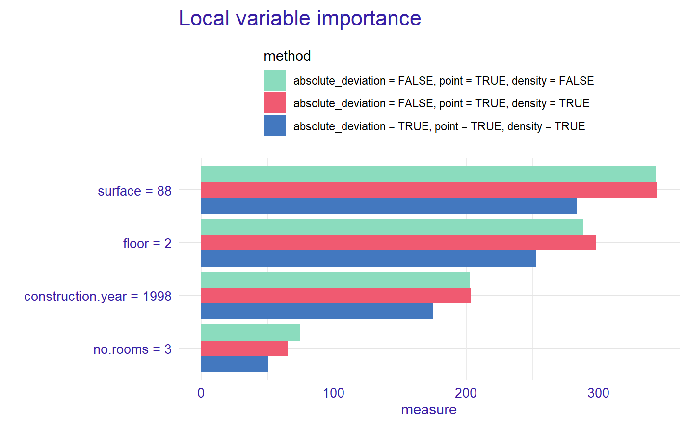
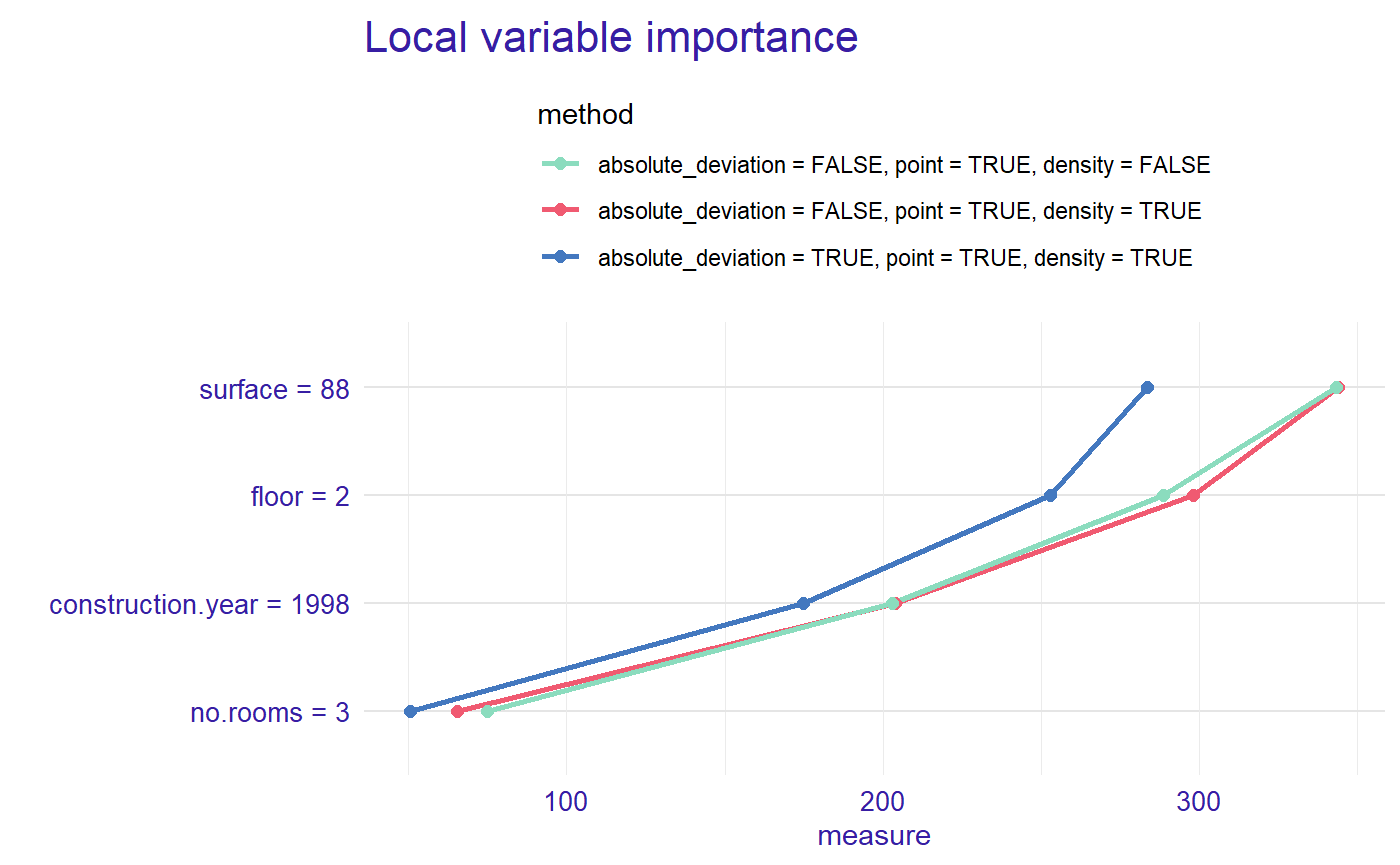
We calculated local variable importance for different parameters and we can plot together, on bar plot or lines plot.

measure_2 <- local_variable_importance(profiles, apartments[,2:5],
            absolute_deviation = FALSE, point = TRUE, density = TRUE)
measure_3 <- local_variable_importance(profiles, apartments[,2:5],
            absolute_deviation = FALSE, point = TRUE, density = FALSE)

plot(measure, measure_2, measure_3, color = "_label_method_")

plot(measure, measure_2, measure_3, color = "_label_method_", type = "lines")

7 Comparison of the importance of variables for two or more models

Let created a linear regression model and explain object.

apartments_lm_model <- lm(m2.price ~ construction.year + surface + floor +
                                      no.rooms, data = apartments)
explainer_lm <- explain(apartments_lm_model,
                        data = apartmentsTest[,2:5], y = apartmentsTest$m2.price)
#> Preparation of a new explainer is initiated
#>   -> model label       :  lm  ( [33m default [39m )
#>   -> data              :  9000  rows  4  cols 
#>   -> target variable   :  9000  values 
#>   -> predict function  :  yhat.lm  will be used ( [33m default [39m )
#>   -> predicted values  :  numerical, min =  2231.8 , mean =  3507.346 , max =  4769.053  
#>   -> model_info        :  package stats , ver. 3.6.3 , task regression ( [33m default [39m ) 
#>   -> residual function :  difference between y and yhat ( [33m default [39m )
#>   -> residuals         :  numerical, min =  -733.2516 , mean =  4.177813 , max =  2107.979  
#>  [32m A new explainer has been created! [39m

We calculated Ceteris Paribus profiles and measure.

profiles_lm <- predict_profile(explainer_lm, new_apartment)

measure_lm <- local_variable_importance(profiles_lm, apartments[,2:5],
            absolute_deviation = TRUE, point = TRUE, density = TRUE)

plot(measure, measure_lm, color = "_label_model_", type = "lines")

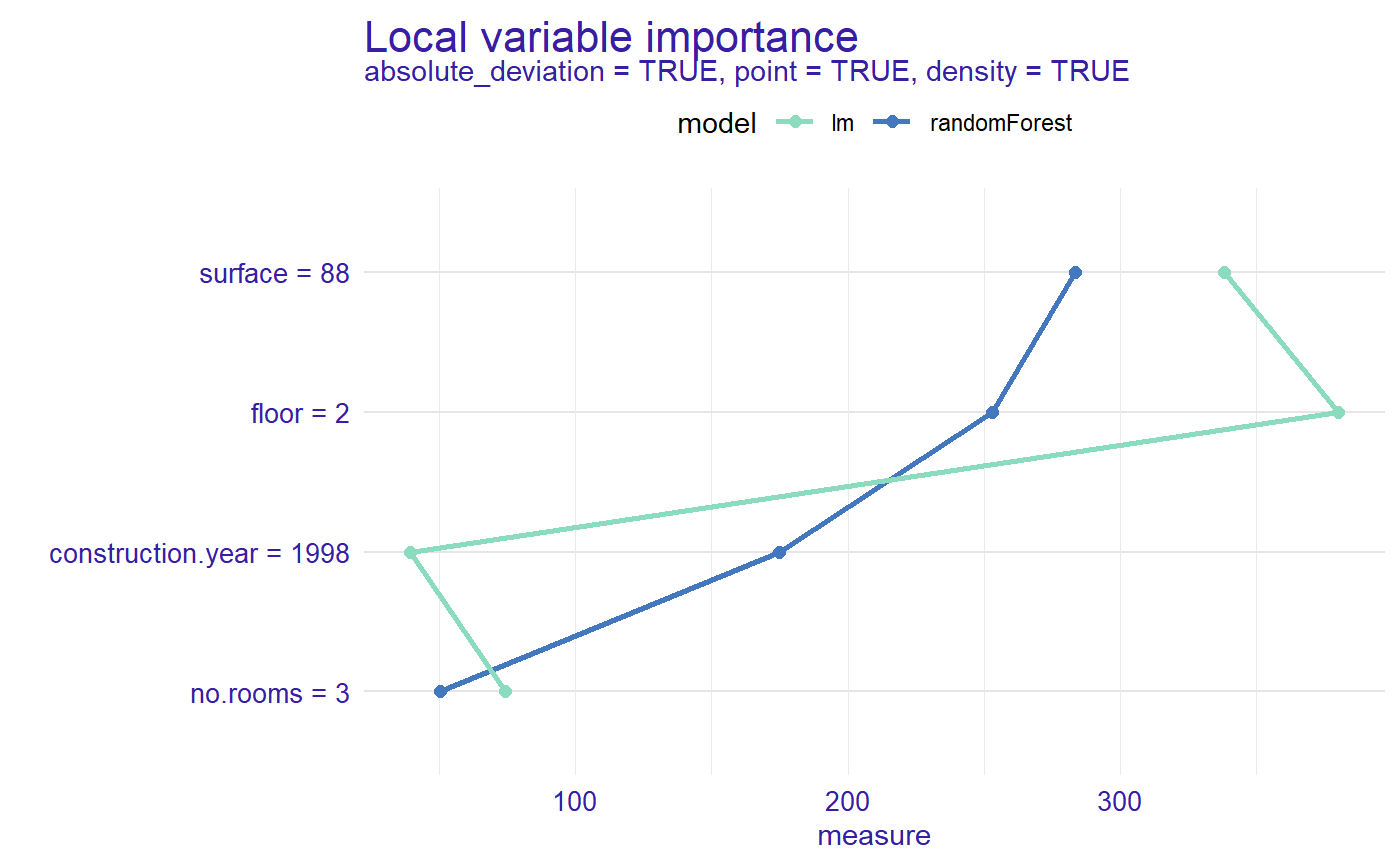
Now we can see the order of importance of variables by model for selected observation.

Example of local variable importance

Anna Kozak

2020-09-26