Plot Generic for Break Down Uncertainty Objects
Source:R/plot_break_down_uncertainty.R
plot.break_down_uncertainty.RdPlot Generic for Break Down Uncertainty Objects
# S3 method for break_down_uncertainty
plot(
  x,
  ...,
  vcolors = DALEX::colors_breakdown_drwhy(),
  show_boxplots = TRUE,
  max_features = 10,
  max_vars = NULL
)
Arguments
- x
an explanation created with
break_down_uncertainty- ...
other parameters.
- vcolors
If
NA(default), DrWhy colors are used.- show_boxplots
logical if
TRUE(default) boxplot will be plotted to show uncertanity of attributions- max_features
maximal number of features to be included in the plot. By default it's
10.- max_vars
alias for the
max_featuresparameter.
Value
a ggplot2 object.
References
Explanatory Model Analysis. Explore, Explain and Examine Predictive Models. https://ema.drwhy.ai
Examples
library("DALEX")
library("iBreakDown")
set.seed(1313)
model_titanic_glm <- glm(survived ~ gender + age + fare,
data = titanic_imputed, family = "binomial")
explain_titanic_glm <- explain(model_titanic_glm,
data = titanic_imputed,
y = titanic_imputed$survived,
label = "glm")
#> Preparation of a new explainer is initiated
#> -> model label : glm
#> -> data : 2207 rows 8 cols
#> -> target variable : 2207 values
#> -> predict function : yhat.glm will be used ( default )
#> -> predicted values : No value for predict function target column. ( default )
#> -> model_info : package stats , ver. 4.1.2 , task classification ( default )
#> -> predicted values : numerical, min = 0.1490412 , mean = 0.3221568 , max = 0.9878987
#> -> residual function : difference between y and yhat ( default )
#> -> residuals : numerical, min = -0.8898433 , mean = 4.198546e-13 , max = 0.8448637
#> A new explainer has been created!
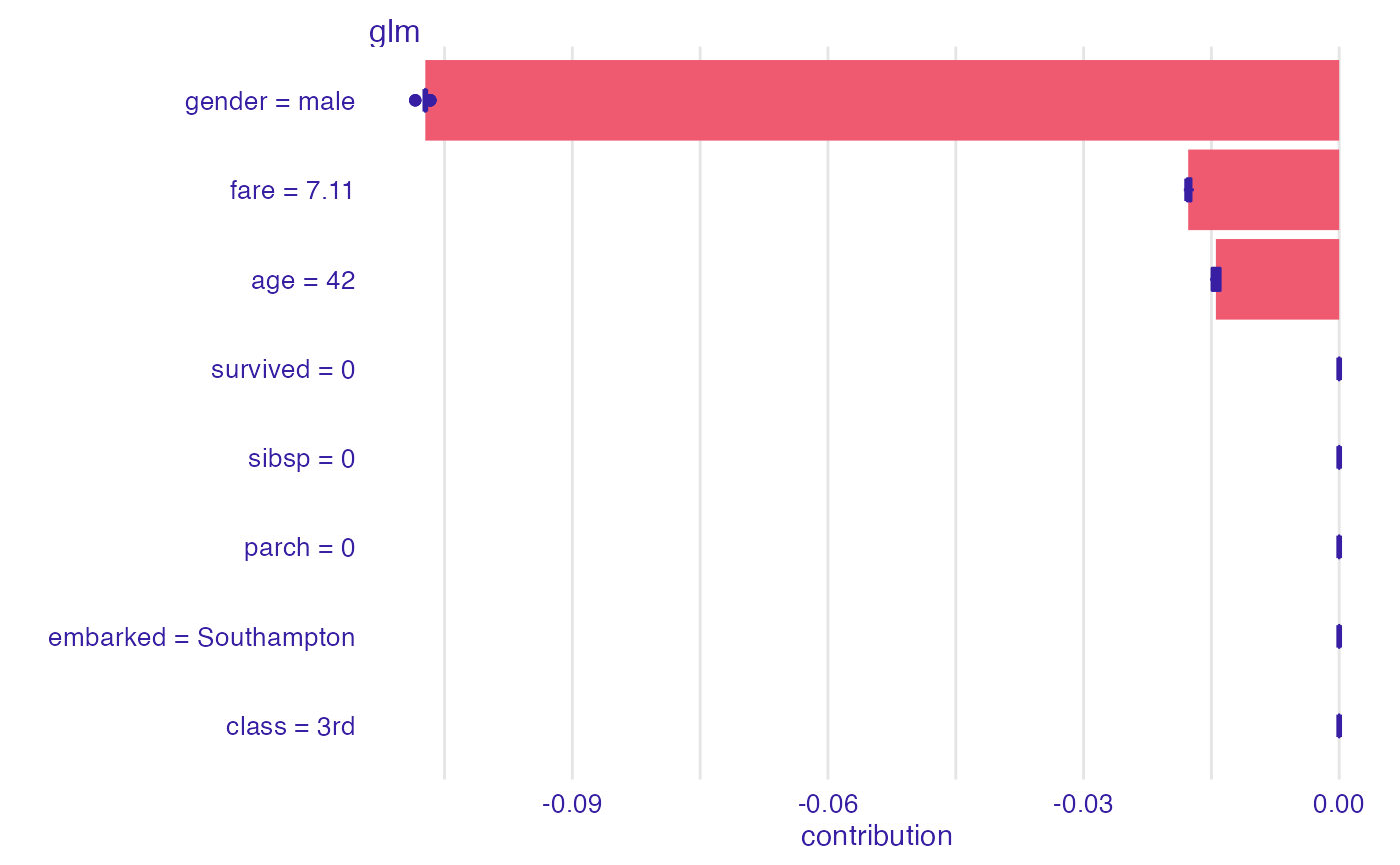
sh_glm <- shap(explain_titanic_glm, titanic_imputed[1, ])
sh_glm
#> min q1 median mean
#> glm: age = 42 -0.01514903 -0.01492541 -0.01434645 -0.01447369
#> glm: class = 3rd 0.00000000 0.00000000 0.00000000 0.00000000
#> glm: embarked = Southampton 0.00000000 0.00000000 0.00000000 0.00000000
#> glm: fare = 7.11 -0.01823177 -0.01784977 -0.01784977 -0.01772034
#> glm: gender = male -0.10843751 -0.10725651 -0.10725651 -0.10725871
#> glm: parch = 0 0.00000000 0.00000000 0.00000000 0.00000000
#> glm: sibsp = 0 0.00000000 0.00000000 0.00000000 0.00000000
#> glm: survived = 0 0.00000000 0.00000000 0.00000000 0.00000000
#> q3 max
#> glm: age = 42 -0.01396446 -0.01396446
#> glm: class = 3rd 0.00000000 0.00000000
#> glm: embarked = Southampton 0.00000000 0.00000000
#> glm: fare = 7.11 -0.01738588 -0.01705077
#> glm: gender = male -0.10725293 -0.10667755
#> glm: parch = 0 0.00000000 0.00000000
#> glm: sibsp = 0 0.00000000 0.00000000
#> glm: survived = 0 0.00000000 0.00000000
plot(sh_glm)
 # \dontrun{
## Not run:
library("randomForest")
set.seed(1313)
model <- randomForest(status ~ . , data = HR)
new_observation <- HR_test[1,]
explainer_rf <- explain(model,
data = HR[1:1000,1:5])
#> Preparation of a new explainer is initiated
#> -> model label : randomForest ( default )
#> -> data : 1000 rows 5 cols
#> -> target variable : not specified! ( WARNING )
#> -> predict function : yhat.randomForest will be used ( default )
#> -> predicted values : No value for predict function target column. ( default )
#> -> model_info : package randomForest , ver. 4.7.1 , task multiclass ( default )
#> -> model_info : Model info detected multiclass task but 'y' is a NULL . ( WARNING )
#> -> model_info : By deafult multiclass tasks supports only factor 'y' parameter.
#> -> model_info : Consider changing to a factor vector with true class names.
#> -> model_info : Otherwise I will not be able to calculate residuals or loss function.
#> -> predicted values : predict function returns multiple columns: 3 ( default )
#> -> residual function : difference between 1 and probability of true class ( default )
#> A new explainer has been created!
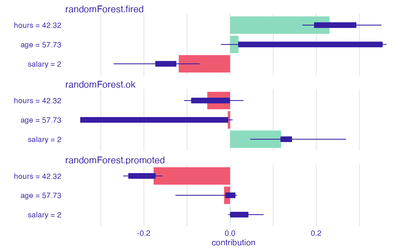
bd_rf <- break_down_uncertainty(explainer_rf,
new_observation,
path = c(3,2,4,1,5),
show_boxplots = FALSE)
bd_rf
#> min q1 median
#> randomForest.fired: age = 57.73 -0.021328 0.019462 0.153816
#> randomForest.fired: evaluation = 2 -0.018856 0.009084 0.035996
#> randomForest.fired: gender = male -0.009380 0.005474 0.019250
#> randomForest.fired: hours = 42.32 0.167650 0.195686 0.230614
#> randomForest.fired: salary = 2 -0.270298 -0.172701 -0.160058
#> randomForest.ok: age = 57.73 -0.346842 -0.346842 -0.162470
#> randomForest.ok: evaluation = 2 0.028666 0.099847 0.125760
#> randomForest.ok: gender = male -0.282642 -0.162907 -0.021756
#> randomForest.ok: hours = 42.32 -0.106876 -0.089536 -0.053010
#> randomForest.ok: salary = 2 0.046824 0.118454 0.118552
#> randomForest.promoted: age = 57.73 -0.126732 -0.010081 -0.006132
#> randomForest.promoted: evaluation = 2 -0.201822 -0.172814 -0.164010
#> randomForest.promoted: gender = male -0.045880 -0.002331 -0.001994
#> randomForest.promoted: hours = 42.32 -0.247972 -0.235271 -0.178676
#> randomForest.promoted: salary = 2 -0.003902 0.001014 0.027152
#> mean q3 max
#> randomForest.fired: age = 57.73 0.178679818 0.352974 0.362800
#> randomForest.fired: evaluation = 2 0.023217636 0.041020 0.045408
#> randomForest.fired: gender = male 0.103037273 0.187181 0.280686
#> randomForest.fired: hours = 42.32 0.244756909 0.291987 0.351330
#> randomForest.fired: salary = 2 -0.157277636 -0.125635 -0.070866
#> randomForest.ok: age = 57.73 -0.167283636 -0.005432 0.005860
#> randomForest.ok: evaluation = 2 0.119492364 0.129860 0.196252
#> randomForest.ok: gender = male -0.096862545 -0.008832 -0.003480
#> randomForest.ok: hours = 42.32 -0.045487455 -0.001451 0.030996
#> randomForest.ok: salary = 2 0.129991273 0.142728 0.268992
#> randomForest.promoted: age = 57.73 -0.011396182 0.011513 0.015468
#> randomForest.promoted: evaluation = 2 -0.142710000 -0.110062 -0.058120
#> randomForest.promoted: gender = male -0.006174727 0.002231 0.023564
#> randomForest.promoted: hours = 42.32 -0.199269455 -0.173865 -0.156930
#> randomForest.promoted: salary = 2 0.027286364 0.041506 0.077562
plot(bd_rf, max_features = 3)
# \dontrun{
## Not run:
library("randomForest")
set.seed(1313)
model <- randomForest(status ~ . , data = HR)
new_observation <- HR_test[1,]
explainer_rf <- explain(model,
data = HR[1:1000,1:5])
#> Preparation of a new explainer is initiated
#> -> model label : randomForest ( default )
#> -> data : 1000 rows 5 cols
#> -> target variable : not specified! ( WARNING )
#> -> predict function : yhat.randomForest will be used ( default )
#> -> predicted values : No value for predict function target column. ( default )
#> -> model_info : package randomForest , ver. 4.7.1 , task multiclass ( default )
#> -> model_info : Model info detected multiclass task but 'y' is a NULL . ( WARNING )
#> -> model_info : By deafult multiclass tasks supports only factor 'y' parameter.
#> -> model_info : Consider changing to a factor vector with true class names.
#> -> model_info : Otherwise I will not be able to calculate residuals or loss function.
#> -> predicted values : predict function returns multiple columns: 3 ( default )
#> -> residual function : difference between 1 and probability of true class ( default )
#> A new explainer has been created!
bd_rf <- break_down_uncertainty(explainer_rf,
new_observation,
path = c(3,2,4,1,5),
show_boxplots = FALSE)
bd_rf
#> min q1 median
#> randomForest.fired: age = 57.73 -0.021328 0.019462 0.153816
#> randomForest.fired: evaluation = 2 -0.018856 0.009084 0.035996
#> randomForest.fired: gender = male -0.009380 0.005474 0.019250
#> randomForest.fired: hours = 42.32 0.167650 0.195686 0.230614
#> randomForest.fired: salary = 2 -0.270298 -0.172701 -0.160058
#> randomForest.ok: age = 57.73 -0.346842 -0.346842 -0.162470
#> randomForest.ok: evaluation = 2 0.028666 0.099847 0.125760
#> randomForest.ok: gender = male -0.282642 -0.162907 -0.021756
#> randomForest.ok: hours = 42.32 -0.106876 -0.089536 -0.053010
#> randomForest.ok: salary = 2 0.046824 0.118454 0.118552
#> randomForest.promoted: age = 57.73 -0.126732 -0.010081 -0.006132
#> randomForest.promoted: evaluation = 2 -0.201822 -0.172814 -0.164010
#> randomForest.promoted: gender = male -0.045880 -0.002331 -0.001994
#> randomForest.promoted: hours = 42.32 -0.247972 -0.235271 -0.178676
#> randomForest.promoted: salary = 2 -0.003902 0.001014 0.027152
#> mean q3 max
#> randomForest.fired: age = 57.73 0.178679818 0.352974 0.362800
#> randomForest.fired: evaluation = 2 0.023217636 0.041020 0.045408
#> randomForest.fired: gender = male 0.103037273 0.187181 0.280686
#> randomForest.fired: hours = 42.32 0.244756909 0.291987 0.351330
#> randomForest.fired: salary = 2 -0.157277636 -0.125635 -0.070866
#> randomForest.ok: age = 57.73 -0.167283636 -0.005432 0.005860
#> randomForest.ok: evaluation = 2 0.119492364 0.129860 0.196252
#> randomForest.ok: gender = male -0.096862545 -0.008832 -0.003480
#> randomForest.ok: hours = 42.32 -0.045487455 -0.001451 0.030996
#> randomForest.ok: salary = 2 0.129991273 0.142728 0.268992
#> randomForest.promoted: age = 57.73 -0.011396182 0.011513 0.015468
#> randomForest.promoted: evaluation = 2 -0.142710000 -0.110062 -0.058120
#> randomForest.promoted: gender = male -0.006174727 0.002231 0.023564
#> randomForest.promoted: hours = 42.32 -0.199269455 -0.173865 -0.156930
#> randomForest.promoted: salary = 2 0.027286364 0.041506 0.077562
plot(bd_rf, max_features = 3)
 # example for regression - apartment prices
# here we do not have intreactions
model <- randomForest(m2.price ~ . , data = apartments)
explainer_rf <- explain(model,
data = apartments_test[1:1000,2:6],
y = apartments_test$m2.price[1:1000])
#> Preparation of a new explainer is initiated
#> -> model label : randomForest ( default )
#> -> data : 1000 rows 5 cols
#> -> target variable : 1000 values
#> -> predict function : yhat.randomForest will be used ( default )
#> -> predicted values : No value for predict function target column. ( default )
#> -> model_info : package randomForest , ver. 4.7.1 , task regression ( default )
#> -> predicted values : numerical, min = 2052.033 , mean = 3487.71 , max = 5776.623
#> -> residual function : difference between y and yhat ( default )
#> -> residuals : numerical, min = -632.8469 , mean = 1.070017 , max = 1328.352
#> A new explainer has been created!
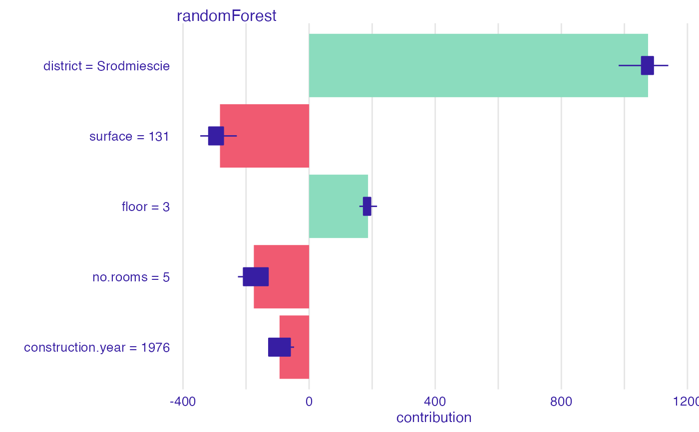
bd_rf <- break_down_uncertainty(explainer_rf,
apartments_test[1,],
path = c("floor", "no.rooms", "district",
"construction.year", "surface"))
bd_rf
#> min q1 median
#> randomForest: construction.year = 1976 -128.5908 -110.1911 -68.37002
#> randomForest: district = Srodmiescie 981.8193 1036.9753 1054.79081
#> randomForest: floor = 3 172.8786 183.5605 193.26996
#> randomForest: no.rooms = 5 -229.8610 -225.7194 -209.30956
#> randomForest: surface = 131 -272.2211 -266.0785 -249.94062
#> mean q3 max
#> randomForest: construction.year = 1976 -81.56069 -52.48483 -47.64365
#> randomForest: district = Srodmiescie 1046.51524 1054.79081 1091.59037
#> randomForest: floor = 3 195.40642 209.02407 215.52532
#> randomForest: no.rooms = 5 -201.00985 -204.86547 -130.21186
#> randomForest: surface = 131 -249.01688 -229.21426 -229.21426
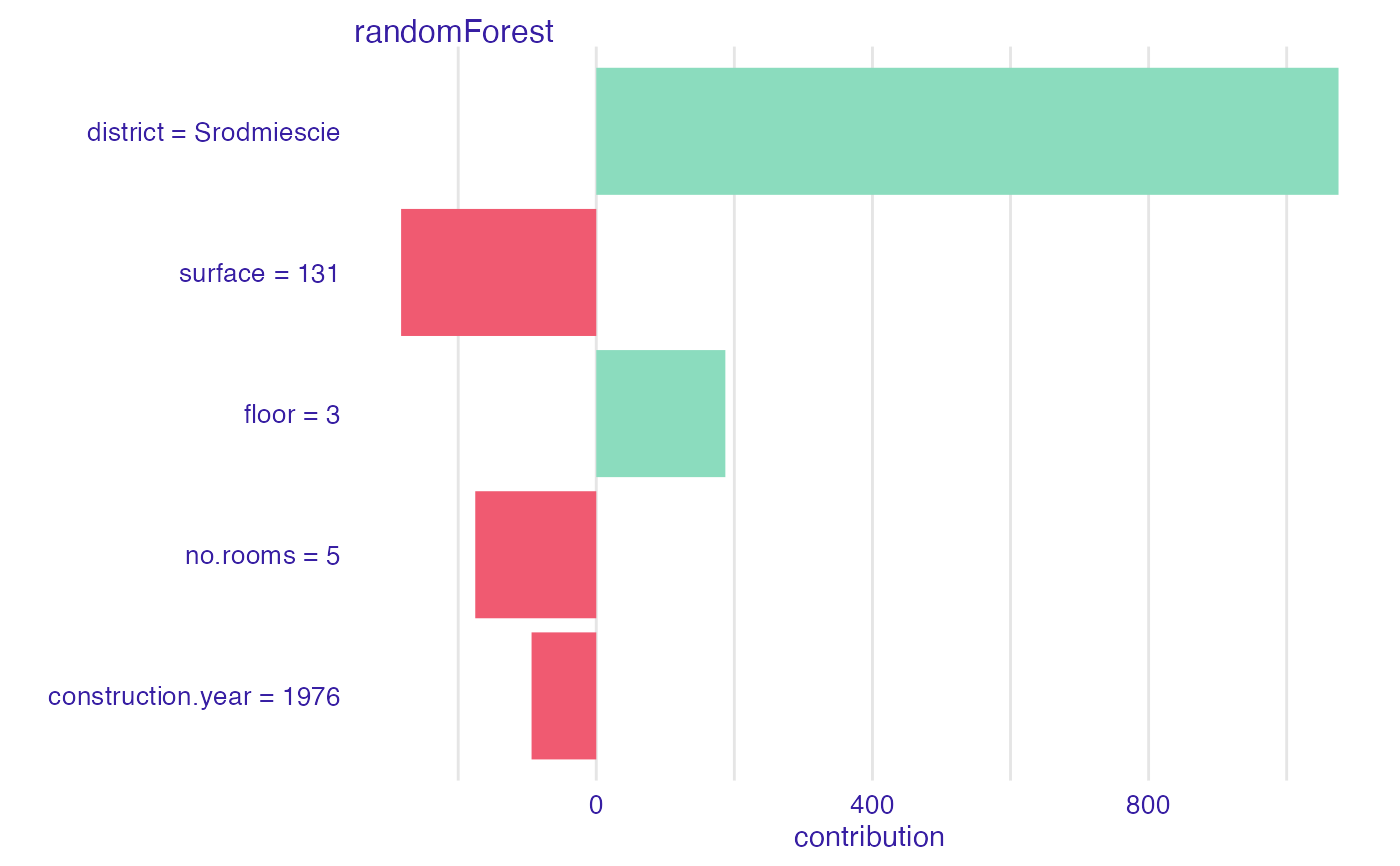
plot(bd_rf)
# example for regression - apartment prices
# here we do not have intreactions
model <- randomForest(m2.price ~ . , data = apartments)
explainer_rf <- explain(model,
data = apartments_test[1:1000,2:6],
y = apartments_test$m2.price[1:1000])
#> Preparation of a new explainer is initiated
#> -> model label : randomForest ( default )
#> -> data : 1000 rows 5 cols
#> -> target variable : 1000 values
#> -> predict function : yhat.randomForest will be used ( default )
#> -> predicted values : No value for predict function target column. ( default )
#> -> model_info : package randomForest , ver. 4.7.1 , task regression ( default )
#> -> predicted values : numerical, min = 2052.033 , mean = 3487.71 , max = 5776.623
#> -> residual function : difference between y and yhat ( default )
#> -> residuals : numerical, min = -632.8469 , mean = 1.070017 , max = 1328.352
#> A new explainer has been created!
bd_rf <- break_down_uncertainty(explainer_rf,
apartments_test[1,],
path = c("floor", "no.rooms", "district",
"construction.year", "surface"))
bd_rf
#> min q1 median
#> randomForest: construction.year = 1976 -128.5908 -110.1911 -68.37002
#> randomForest: district = Srodmiescie 981.8193 1036.9753 1054.79081
#> randomForest: floor = 3 172.8786 183.5605 193.26996
#> randomForest: no.rooms = 5 -229.8610 -225.7194 -209.30956
#> randomForest: surface = 131 -272.2211 -266.0785 -249.94062
#> mean q3 max
#> randomForest: construction.year = 1976 -81.56069 -52.48483 -47.64365
#> randomForest: district = Srodmiescie 1046.51524 1054.79081 1091.59037
#> randomForest: floor = 3 195.40642 209.02407 215.52532
#> randomForest: no.rooms = 5 -201.00985 -204.86547 -130.21186
#> randomForest: surface = 131 -249.01688 -229.21426 -229.21426
plot(bd_rf)
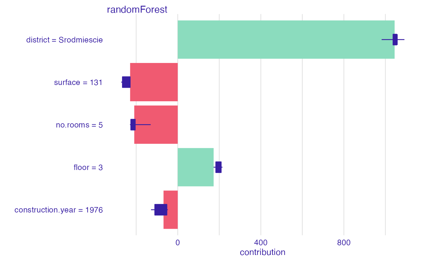 bd_rf <- shap(explainer_rf,
apartments_test[1,])
bd_rf
#> min q1 median
#> randomForest: construction.year = 1976 -128.5908 -127.7759 -92.75977
#> randomForest: district = Srodmiescie 981.8193 1054.7908 1069.75828
#> randomForest: floor = 3 159.4690 172.8786 184.31616
#> randomForest: no.rooms = 5 -225.7194 -207.9039 -198.81536
#> randomForest: surface = 131 -345.1926 -318.0552 -277.00849
#> mean q3 max
#> randomForest: construction.year = 1976 -93.72824 -60.08701 -47.64365
#> randomForest: district = Srodmiescie 1075.07584 1091.59037 1139.28110
#> randomForest: floor = 3 186.95249 194.98506 215.52532
#> randomForest: no.rooms = 5 -175.28235 -130.21186 -130.21186
#> randomForest: surface = 131 -282.68349 -272.14890 -229.21426
plot(bd_rf)
bd_rf <- shap(explainer_rf,
apartments_test[1,])
bd_rf
#> min q1 median
#> randomForest: construction.year = 1976 -128.5908 -127.7759 -92.75977
#> randomForest: district = Srodmiescie 981.8193 1054.7908 1069.75828
#> randomForest: floor = 3 159.4690 172.8786 184.31616
#> randomForest: no.rooms = 5 -225.7194 -207.9039 -198.81536
#> randomForest: surface = 131 -345.1926 -318.0552 -277.00849
#> mean q3 max
#> randomForest: construction.year = 1976 -93.72824 -60.08701 -47.64365
#> randomForest: district = Srodmiescie 1075.07584 1091.59037 1139.28110
#> randomForest: floor = 3 186.95249 194.98506 215.52532
#> randomForest: no.rooms = 5 -175.28235 -130.21186 -130.21186
#> randomForest: surface = 131 -282.68349 -272.14890 -229.21426
plot(bd_rf)
 plot(bd_rf, show_boxplots = FALSE)
 # }
# }