Displays a waterfall break down plot for objects of break_down class.
# S3 method for break_down
plot(
  x,
  ...,
  baseline = NA,
  max_features = 10,
  min_max = NA,
  vcolors = DALEX::colors_breakdown_drwhy(),
  digits = 3,
  rounding_function = round,
  add_contributions = TRUE,
  shift_contributions = 0.05,
  plot_distributions = FALSE,
  vnames = NULL,
  title = "Break Down profile",
  subtitle = "",
  max_vars = NULL
)
Arguments
- x
an explanation created with
break_down- ...
other parameters.
- baseline
if numeric then veritical line starts in
baseline.- max_features
maximal number of features to be included in the plot. default value is
10.- min_max
a range of OX axis. By default
NA, therefore it will be extracted from the contributions ofx. But it can be set to some constants, useful if these plots are to be used for comparisons.- vcolors
If
NA(default), DrWhy colors are used.- digits
number of decimal places (
round) or significant digits (signif) to be used. See therounding_functionargument.- rounding_function
a function to be used for rounding numbers. This should be
signifwhich keeps a specified number of significant digits orround(which is default) to have the same precision for all components.- add_contributions
if
TRUE, variable contributions will be added to the plot- shift_contributions
number describing how much labels should be shifted to the right, as a fraction of range. By default equal to
0.05.- plot_distributions
if
TRUEthen distributions of conditional propotions will be plotted. This requireskeep_distributions=TRUEin thebreak_down,local_attributions, orlocal_interactions.- vnames
a character vector, if specified then will be used as labels on OY axis. By default NULL
- title
a character. Plot title. By default
"Break Down profile".- subtitle
a character. Plot subtitle. By default
"".- max_vars
alias for the
max_featuresparameter.
Value
a ggplot2 object.
References
Explanatory Model Analysis. Explore, Explain and Examine Predictive Models. https://ema.drwhy.ai
Examples
library("DALEX")
library("iBreakDown")
set.seed(1313)
model_titanic_glm <- glm(survived ~ gender + age + fare,
data = titanic_imputed, family = "binomial")
explain_titanic_glm <- explain(model_titanic_glm,
data = titanic_imputed,
y = titanic_imputed$survived,
label = "glm")
#> Preparation of a new explainer is initiated
#> -> model label : glm
#> -> data : 2207 rows 8 cols
#> -> target variable : 2207 values
#> -> predict function : yhat.glm will be used ( default )
#> -> predicted values : No value for predict function target column. ( default )
#> -> model_info : package stats , ver. 4.1.2 , task classification ( default )
#> -> predicted values : numerical, min = 0.1490412 , mean = 0.3221568 , max = 0.9878987
#> -> residual function : difference between y and yhat ( default )
#> -> residuals : numerical, min = -0.8898433 , mean = 4.198546e-13 , max = 0.8448637
#> A new explainer has been created!
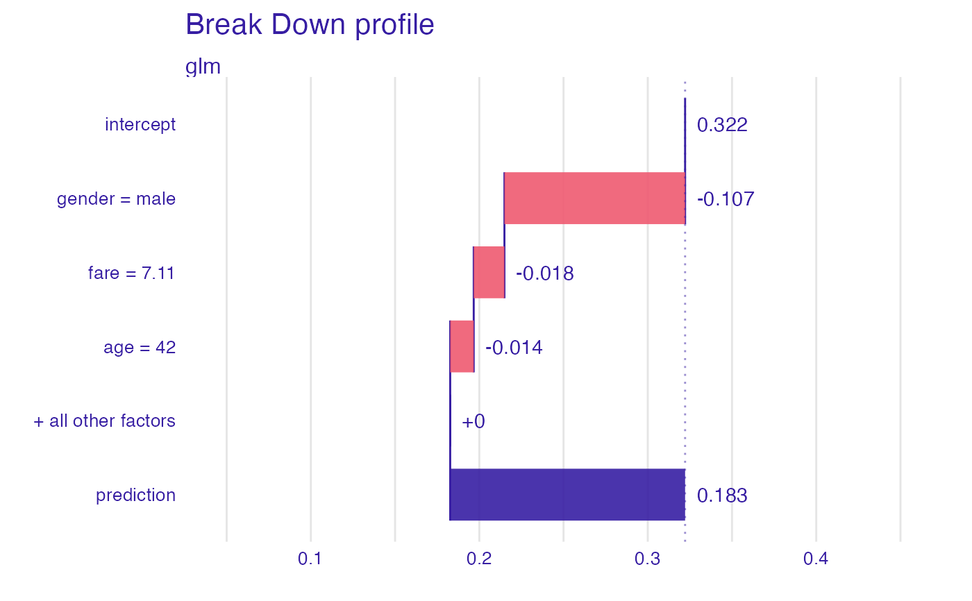
bd_glm <- break_down(explain_titanic_glm, titanic_imputed[1, ])
bd_glm
#> contribution
#> glm: intercept 0.322
#> glm: gender = male -0.107
#> glm: fare = 7.11 -0.018
#> glm: age = 42 -0.014
#> glm: class = 3rd 0.000
#> glm: embarked = Southampton 0.000
#> glm: sibsp = 0 0.000
#> glm: parch = 0 0.000
#> glm: survived = 0 0.000
#> glm: prediction 0.183
plot(bd_glm, max_features = 3)
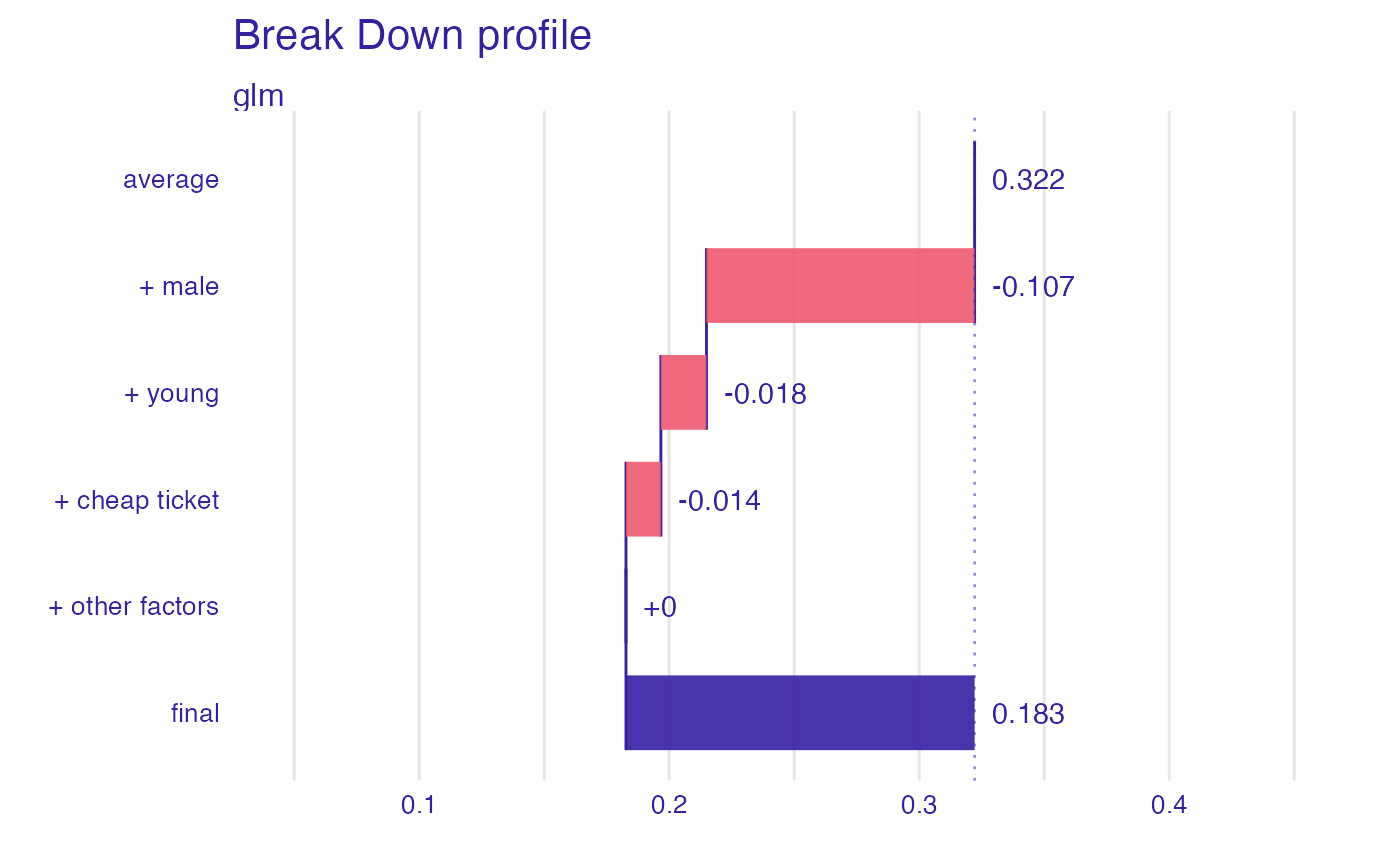
 plot(bd_glm, max_features = 3,
vnames = c("average","+ male","+ young","+ cheap ticket", "+ other factors", "final"))
plot(bd_glm, max_features = 3,
vnames = c("average","+ male","+ young","+ cheap ticket", "+ other factors", "final"))
 # \dontrun{
## Not run:
library("randomForest")
set.seed(1313)
# example with interaction
# classification for HR data
model <- randomForest(status ~ . , data = HR)
new_observation <- HR_test[1,]
explainer_rf <- explain(model,
data = HR[1:1000,1:5])
#> Preparation of a new explainer is initiated
#> -> model label : randomForest ( default )
#> -> data : 1000 rows 5 cols
#> -> target variable : not specified! ( WARNING )
#> -> predict function : yhat.randomForest will be used ( default )
#> -> predicted values : No value for predict function target column. ( default )
#> -> model_info : package randomForest , ver. 4.7.1 , task multiclass ( default )
#> -> model_info : Model info detected multiclass task but 'y' is a NULL . ( WARNING )
#> -> model_info : By deafult multiclass tasks supports only factor 'y' parameter.
#> -> model_info : Consider changing to a factor vector with true class names.
#> -> model_info : Otherwise I will not be able to calculate residuals or loss function.
#> -> predicted values : predict function returns multiple columns: 3 ( default )
#> -> residual function : difference between 1 and probability of true class ( default )
#> A new explainer has been created!
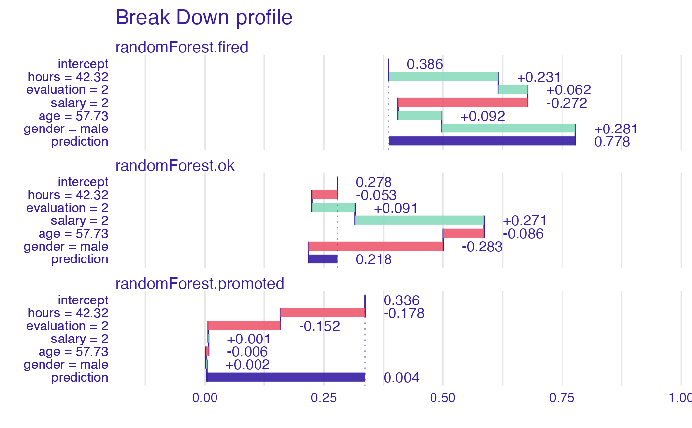
bd_rf <- local_attributions(explainer_rf,
new_observation)
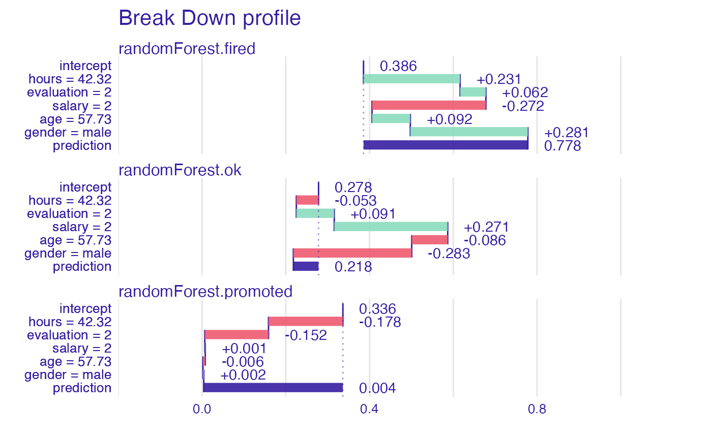
bd_rf
#> contribution
#> randomForest.fired: intercept 0.386
#> randomForest.fired: hours = 42.32 0.231
#> randomForest.fired: evaluation = 2 0.062
#> randomForest.fired: salary = 2 -0.272
#> randomForest.fired: age = 57.73 0.092
#> randomForest.fired: gender = male 0.281
#> randomForest.fired: prediction 0.778
#> randomForest.ok: intercept 0.278
#> randomForest.ok: hours = 42.32 -0.053
#> randomForest.ok: evaluation = 2 0.091
#> randomForest.ok: salary = 2 0.271
#> randomForest.ok: age = 57.73 -0.086
#> randomForest.ok: gender = male -0.283
#> randomForest.ok: prediction 0.218
#> randomForest.promoted: intercept 0.336
#> randomForest.promoted: hours = 42.32 -0.178
#> randomForest.promoted: evaluation = 2 -0.152
#> randomForest.promoted: salary = 2 0.001
#> randomForest.promoted: age = 57.73 -0.006
#> randomForest.promoted: gender = male 0.002
#> randomForest.promoted: prediction 0.004
plot(bd_rf)
# \dontrun{
## Not run:
library("randomForest")
set.seed(1313)
# example with interaction
# classification for HR data
model <- randomForest(status ~ . , data = HR)
new_observation <- HR_test[1,]
explainer_rf <- explain(model,
data = HR[1:1000,1:5])
#> Preparation of a new explainer is initiated
#> -> model label : randomForest ( default )
#> -> data : 1000 rows 5 cols
#> -> target variable : not specified! ( WARNING )
#> -> predict function : yhat.randomForest will be used ( default )
#> -> predicted values : No value for predict function target column. ( default )
#> -> model_info : package randomForest , ver. 4.7.1 , task multiclass ( default )
#> -> model_info : Model info detected multiclass task but 'y' is a NULL . ( WARNING )
#> -> model_info : By deafult multiclass tasks supports only factor 'y' parameter.
#> -> model_info : Consider changing to a factor vector with true class names.
#> -> model_info : Otherwise I will not be able to calculate residuals or loss function.
#> -> predicted values : predict function returns multiple columns: 3 ( default )
#> -> residual function : difference between 1 and probability of true class ( default )
#> A new explainer has been created!
bd_rf <- local_attributions(explainer_rf,
new_observation)
bd_rf
#> contribution
#> randomForest.fired: intercept 0.386
#> randomForest.fired: hours = 42.32 0.231
#> randomForest.fired: evaluation = 2 0.062
#> randomForest.fired: salary = 2 -0.272
#> randomForest.fired: age = 57.73 0.092
#> randomForest.fired: gender = male 0.281
#> randomForest.fired: prediction 0.778
#> randomForest.ok: intercept 0.278
#> randomForest.ok: hours = 42.32 -0.053
#> randomForest.ok: evaluation = 2 0.091
#> randomForest.ok: salary = 2 0.271
#> randomForest.ok: age = 57.73 -0.086
#> randomForest.ok: gender = male -0.283
#> randomForest.ok: prediction 0.218
#> randomForest.promoted: intercept 0.336
#> randomForest.promoted: hours = 42.32 -0.178
#> randomForest.promoted: evaluation = 2 -0.152
#> randomForest.promoted: salary = 2 0.001
#> randomForest.promoted: age = 57.73 -0.006
#> randomForest.promoted: gender = male 0.002
#> randomForest.promoted: prediction 0.004
plot(bd_rf)
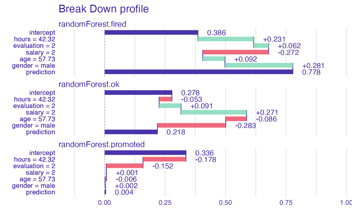
 plot(bd_rf, baseline = 0)
 plot(bd_rf, min_max = c(0,1))
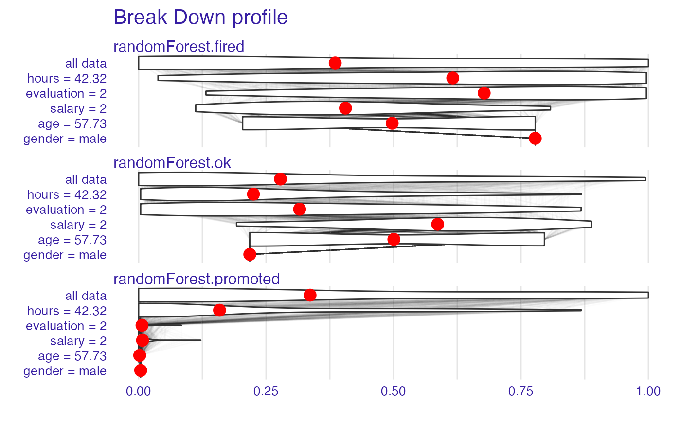
 bd_rf <- local_attributions(explainer_rf,
new_observation,
keep_distributions = TRUE)
bd_rf
#> contribution
#> randomForest.fired: intercept 0.386
#> randomForest.fired: hours = 42.32 0.231
#> randomForest.fired: evaluation = 2 0.062
#> randomForest.fired: salary = 2 -0.272
#> randomForest.fired: age = 57.73 0.092
#> randomForest.fired: gender = male 0.281
#> randomForest.fired: prediction 0.778
#> randomForest.ok: intercept 0.278
#> randomForest.ok: hours = 42.32 -0.053
#> randomForest.ok: evaluation = 2 0.091
#> randomForest.ok: salary = 2 0.271
#> randomForest.ok: age = 57.73 -0.086
#> randomForest.ok: gender = male -0.283
#> randomForest.ok: prediction 0.218
#> randomForest.promoted: intercept 0.336
#> randomForest.promoted: hours = 42.32 -0.178
#> randomForest.promoted: evaluation = 2 -0.152
#> randomForest.promoted: salary = 2 0.001
#> randomForest.promoted: age = 57.73 -0.006
#> randomForest.promoted: gender = male 0.002
#> randomForest.promoted: prediction 0.004
plot(bd_rf, plot_distributions = TRUE)
#> Warning: `fun.y` is deprecated. Use `fun` instead.
bd_rf <- local_attributions(explainer_rf,
new_observation,
keep_distributions = TRUE)
bd_rf
#> contribution
#> randomForest.fired: intercept 0.386
#> randomForest.fired: hours = 42.32 0.231
#> randomForest.fired: evaluation = 2 0.062
#> randomForest.fired: salary = 2 -0.272
#> randomForest.fired: age = 57.73 0.092
#> randomForest.fired: gender = male 0.281
#> randomForest.fired: prediction 0.778
#> randomForest.ok: intercept 0.278
#> randomForest.ok: hours = 42.32 -0.053
#> randomForest.ok: evaluation = 2 0.091
#> randomForest.ok: salary = 2 0.271
#> randomForest.ok: age = 57.73 -0.086
#> randomForest.ok: gender = male -0.283
#> randomForest.ok: prediction 0.218
#> randomForest.promoted: intercept 0.336
#> randomForest.promoted: hours = 42.32 -0.178
#> randomForest.promoted: evaluation = 2 -0.152
#> randomForest.promoted: salary = 2 0.001
#> randomForest.promoted: age = 57.73 -0.006
#> randomForest.promoted: gender = male 0.002
#> randomForest.promoted: prediction 0.004
plot(bd_rf, plot_distributions = TRUE)
#> Warning: `fun.y` is deprecated. Use `fun` instead.
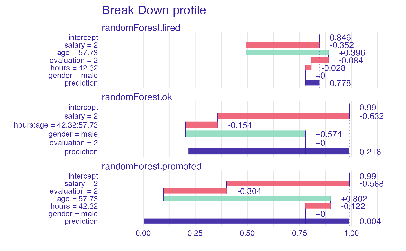
 bd_rf <- local_interactions(explainer_rf,
new_observation,
keep_distributions = TRUE)
bd_rf
#> contribution
#> randomForest.fired: intercept 0.846
#> randomForest.fired: salary = 2 -0.352
#> randomForest.fired: age = 57.73 0.396
#> randomForest.fired: evaluation = 2 -0.084
#> randomForest.fired: hours = 42.32 -0.028
#> randomForest.fired: gender = male 0.000
#> randomForest.fired: prediction 0.778
#> randomForest.ok: intercept 0.990
#> randomForest.ok: salary = 2 -0.632
#> randomForest.ok: hours:age = 42.32:57.73 -0.154
#> randomForest.ok: gender = male 0.574
#> randomForest.ok: evaluation = 2 0.000
#> randomForest.ok: prediction 0.218
#> randomForest.promoted: intercept 0.990
#> randomForest.promoted: salary = 2 -0.588
#> randomForest.promoted: evaluation = 2 -0.304
#> randomForest.promoted: age = 57.73 0.802
#> randomForest.promoted: hours = 42.32 -0.122
#> randomForest.promoted: gender = male 0.000
#> randomForest.promoted: prediction 0.004
plot(bd_rf)
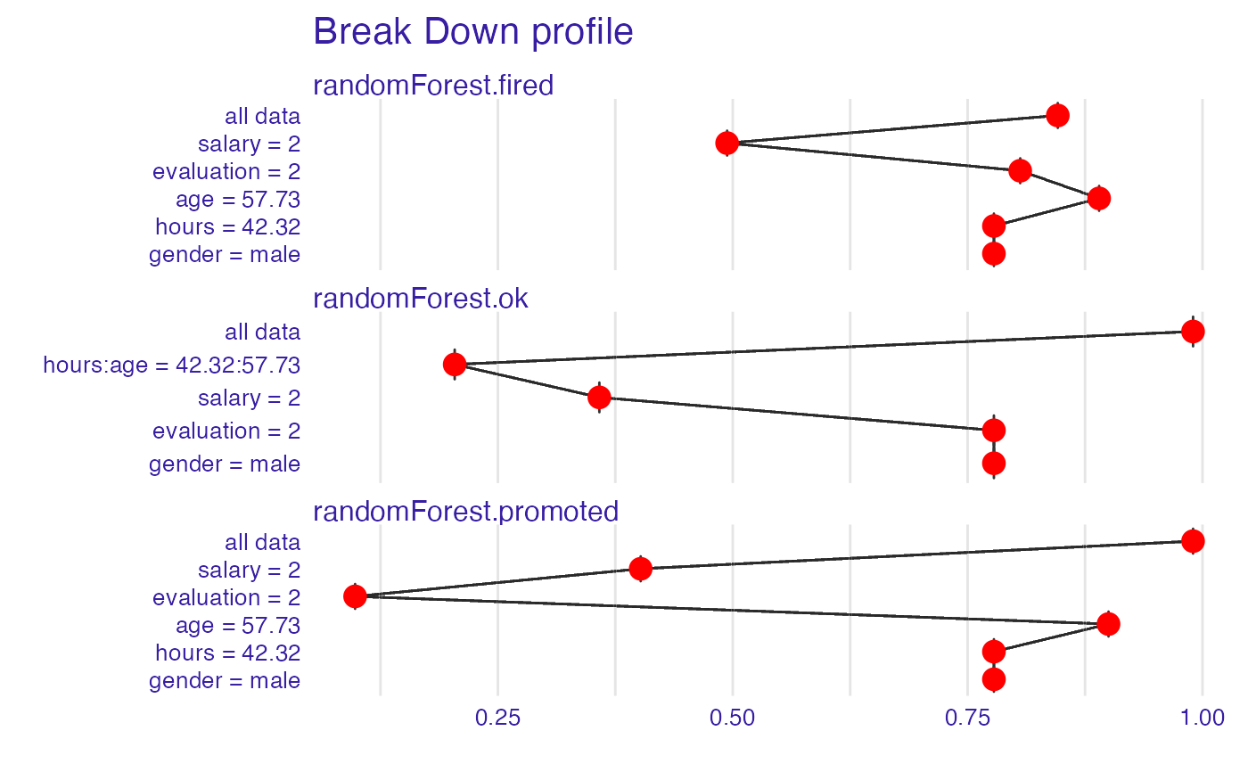
bd_rf <- local_interactions(explainer_rf,
new_observation,
keep_distributions = TRUE)
bd_rf
#> contribution
#> randomForest.fired: intercept 0.846
#> randomForest.fired: salary = 2 -0.352
#> randomForest.fired: age = 57.73 0.396
#> randomForest.fired: evaluation = 2 -0.084
#> randomForest.fired: hours = 42.32 -0.028
#> randomForest.fired: gender = male 0.000
#> randomForest.fired: prediction 0.778
#> randomForest.ok: intercept 0.990
#> randomForest.ok: salary = 2 -0.632
#> randomForest.ok: hours:age = 42.32:57.73 -0.154
#> randomForest.ok: gender = male 0.574
#> randomForest.ok: evaluation = 2 0.000
#> randomForest.ok: prediction 0.218
#> randomForest.promoted: intercept 0.990
#> randomForest.promoted: salary = 2 -0.588
#> randomForest.promoted: evaluation = 2 -0.304
#> randomForest.promoted: age = 57.73 0.802
#> randomForest.promoted: hours = 42.32 -0.122
#> randomForest.promoted: gender = male 0.000
#> randomForest.promoted: prediction 0.004
plot(bd_rf)
 plot(bd_rf, plot_distributions = TRUE)
#> Warning: `fun.y` is deprecated. Use `fun` instead.
plot(bd_rf, plot_distributions = TRUE)
#> Warning: `fun.y` is deprecated. Use `fun` instead.
 # example for regression - apartment prices
# here we do not have intreactions
model <- randomForest(m2.price ~ . , data = apartments)
explainer_rf <- explain(model,
data = apartments_test[1:1000,2:6],
y = apartments_test$m2.price[1:1000])
#> Preparation of a new explainer is initiated
#> -> model label : randomForest ( default )
#> -> data : 1000 rows 5 cols
#> -> target variable : 1000 values
#> -> predict function : yhat.randomForest will be used ( default )
#> -> predicted values : No value for predict function target column. ( default )
#> -> model_info : package randomForest , ver. 4.7.1 , task regression ( default )
#> -> predicted values : numerical, min = 2043.066 , mean = 3487.722 , max = 5773.976
#> -> residual function : difference between y and yhat ( default )
#> -> residuals : numerical, min = -630.6766 , mean = 1.057813 , max = 1256.239
#> A new explainer has been created!
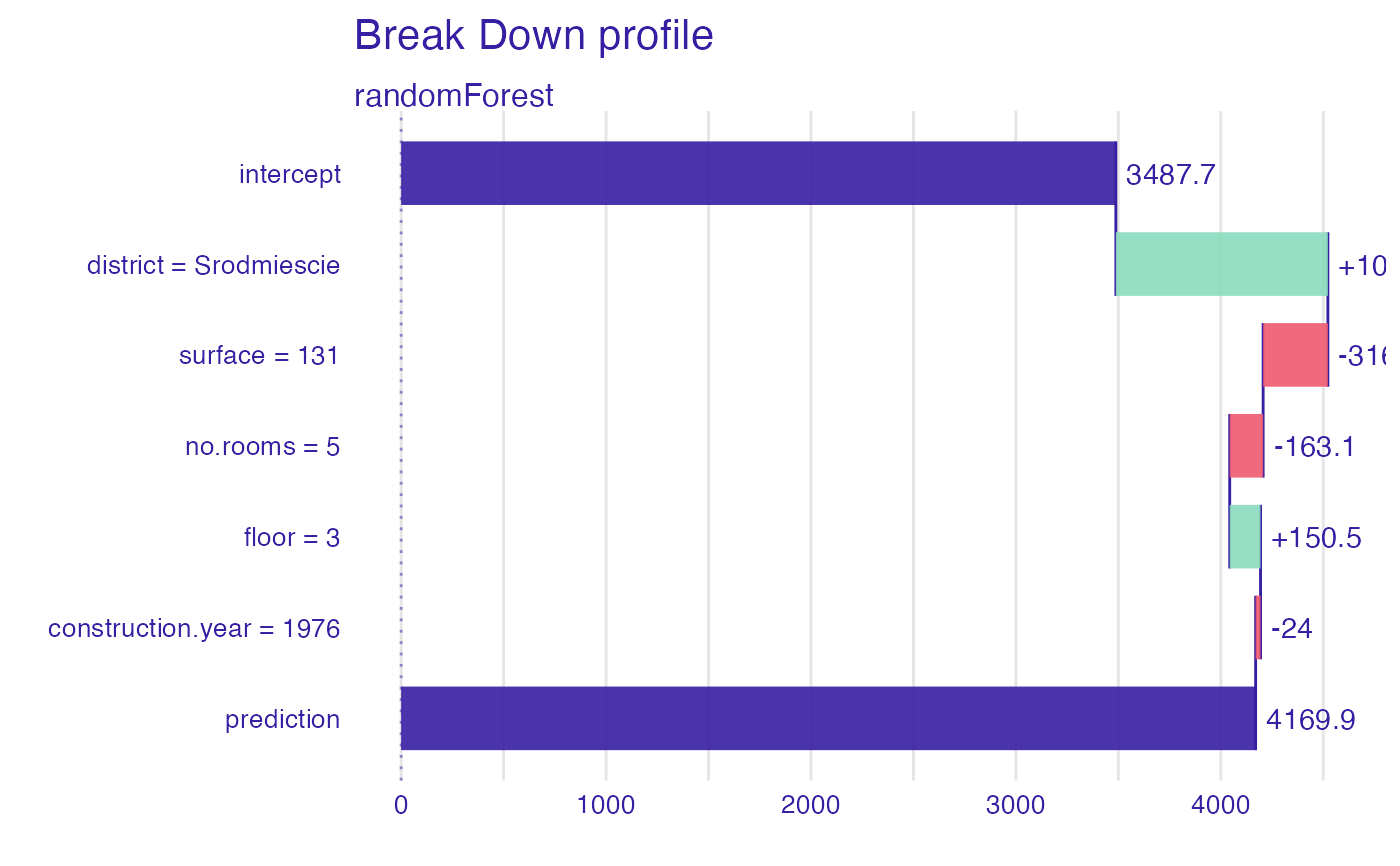
bd_rf <- local_attributions(explainer_rf,
apartments_test[1,])
bd_rf
#> contribution
#> randomForest: intercept 3487.722
#> randomForest: district = Srodmiescie 1034.737
#> randomForest: surface = 131 -315.991
#> randomForest: no.rooms = 5 -163.113
#> randomForest: floor = 3 150.529
#> randomForest: construction.year = 1976 -24.021
#> randomForest: prediction 4169.863
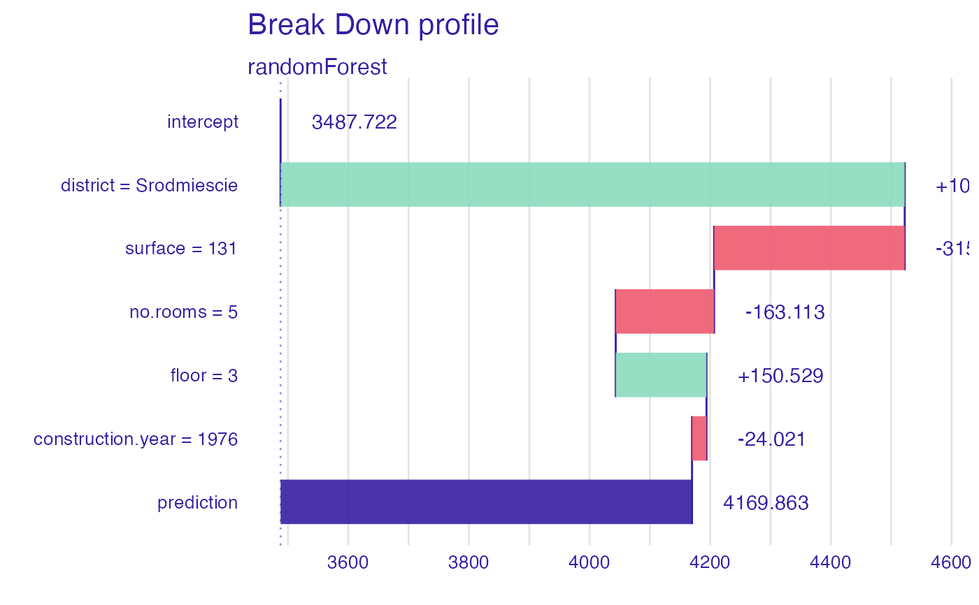
plot(bd_rf, digits = 1)
# example for regression - apartment prices
# here we do not have intreactions
model <- randomForest(m2.price ~ . , data = apartments)
explainer_rf <- explain(model,
data = apartments_test[1:1000,2:6],
y = apartments_test$m2.price[1:1000])
#> Preparation of a new explainer is initiated
#> -> model label : randomForest ( default )
#> -> data : 1000 rows 5 cols
#> -> target variable : 1000 values
#> -> predict function : yhat.randomForest will be used ( default )
#> -> predicted values : No value for predict function target column. ( default )
#> -> model_info : package randomForest , ver. 4.7.1 , task regression ( default )
#> -> predicted values : numerical, min = 2043.066 , mean = 3487.722 , max = 5773.976
#> -> residual function : difference between y and yhat ( default )
#> -> residuals : numerical, min = -630.6766 , mean = 1.057813 , max = 1256.239
#> A new explainer has been created!
bd_rf <- local_attributions(explainer_rf,
apartments_test[1,])
bd_rf
#> contribution
#> randomForest: intercept 3487.722
#> randomForest: district = Srodmiescie 1034.737
#> randomForest: surface = 131 -315.991
#> randomForest: no.rooms = 5 -163.113
#> randomForest: floor = 3 150.529
#> randomForest: construction.year = 1976 -24.021
#> randomForest: prediction 4169.863
plot(bd_rf, digits = 1)
 plot(bd_rf, digits = 1, baseline = 0)
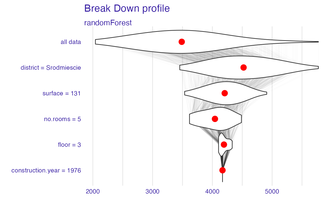
 bd_rf <- local_attributions(explainer_rf,
apartments_test[1,],
keep_distributions = TRUE)
plot(bd_rf, plot_distributions = TRUE)
#> Warning: `fun.y` is deprecated. Use `fun` instead.
bd_rf <- local_attributions(explainer_rf,
apartments_test[1,],
keep_distributions = TRUE)
plot(bd_rf, plot_distributions = TRUE)
#> Warning: `fun.y` is deprecated. Use `fun` instead.
 bd_rf <- local_interactions(explainer_rf,
new_observation = apartments_test[1,],
keep_distributions = TRUE)
bd_rf
#> contribution
#> randomForest: intercept 3487.722
#> randomForest: district = Srodmiescie 1034.737
#> randomForest: surface = 131 -315.991
#> randomForest: no.rooms = 5 -163.113
#> randomForest: floor = 3 150.529
#> randomForest: construction.year = 1976 -24.021
#> randomForest: prediction 4169.863
plot(bd_rf)
bd_rf <- local_interactions(explainer_rf,
new_observation = apartments_test[1,],
keep_distributions = TRUE)
bd_rf
#> contribution
#> randomForest: intercept 3487.722
#> randomForest: district = Srodmiescie 1034.737
#> randomForest: surface = 131 -315.991
#> randomForest: no.rooms = 5 -163.113
#> randomForest: floor = 3 150.529
#> randomForest: construction.year = 1976 -24.021
#> randomForest: prediction 4169.863
plot(bd_rf)
 plot(bd_rf, plot_distributions = TRUE)
#> Warning: `fun.y` is deprecated. Use `fun` instead.
plot(bd_rf, plot_distributions = TRUE)
#> Warning: `fun.y` is deprecated. Use `fun` instead.
 # }
# }