Instance Level Parts of Survival Model Predictions

This function decomposes the model prediction into individual parts, which are attributions of particular variables. The explanations can be made via the SurvLIME and SurvSHAP(t) methods.

predict_parts(explainer, ...)

# S3 method for surv_explainer
predict_parts(
  explainer,
  new_observation,
  ...,
  N = NULL,
  type = "survshap",
  output_type = "survival",
  explanation_label = NULL
)

Arguments

explainer: an explainer object - model preprocessed by the explain() function
...: other parameters which are passed to iBreakDown::break_down if output_type=="risk", or if output_type=="survival" to surv_shap() or surv_lime() functions depending on the selected type
new_observation: a new observation for which prediction need to be explained
N: the number of observations used for calculation of attributions. If NULL (default) all explainer data will be used for SurvSHAP(t) and 100 neigbours for SurvLIME.
type: if output_type == "survival" must be either "survshap" or "survlime", otherwise refer to the DALEX::predict_parts
output_type: either "survival", "chf" or "risk" the type of survival model output that should be considered for explanations. If "survival" the explanations are based on the survival function. If "chf" the explanations are based on the cumulative hazard function. Otherwise the scalar risk predictions are used by the DALEX::predict_parts function.
explanation_label: a label that can overwrite explainer label (useful for multiple explanations for the same explainer/model)

Value

An object of class "predict_parts_survival" and additional classes depending on the type of explanations. It is a list with the element result containing the results of the calculation.

Additional parameters

There are additional parameters that are passed to internal functions

for survlime
- N - a positive integer, number of observations generated in the neighbourhood
- distance_metric - character, name of the distance metric to be used, only "euclidean" is implemented
- kernel_width - a numeric or "silverman", parameter used for calculating weights, by default it's sqrt(ncol(data)*0.75). If "silverman" the kernel width is calculated using the method proposed by Silverman and used in the SurvLIMEpy Python package.
- sampling_method - character, name of the method of generating neighbourhood, only "gaussian" is implemented
- sample_around_instance - logical, if the neighbourhood should be generated with the new observation as the center (default), or should the mean of the whole dataset be used as the center
- max_iter - a numeric, maximal number of iteration for the optimization problem
- categorical_variables - character vector, names of variables that should be treated as categories (factors are included by default)
- k - a small positive number > 1, added to chf before taking log, so that weigths aren't negative
for survshap
- y_true - a two element numeric vector or matrix of one row and two columns, the first element being the true observed time and the second the status of the observation, used for plotting
- calculation_method - a character, either "kernelshap" for use of kernelshap library (providing faster Kernel SHAP with refinements) or "exact_kernel" for exact Kernel SHAP estimation
- aggregation_method - a character, either "mean_absolute" or "integral", "max_absolute", "sum_of_squares"

References

[1] Krzyziński, Mateusz, et al. "SurvSHAP(t): Time-dependent explanations of machine learning survival models." Knowledge-Based Systems 262 (2023): 110234
[2] Kovalev, Maxim S., et al. "SurvLIME: A method for explaining machine learning survival models." Knowledge-Based Systems 203 (2020): 106164.
[3] Pachón-García, Cristian, et al. "SurvLIMEpy: A Python package implementing SurvLIME." Expert Systems with Applications 237 (2024): 121620.

Examples

# \donttest{
library(survival)
library(survex)

cph <- coxph(Surv(time, status) ~ ., data = veteran, model = TRUE, x = TRUE, y = TRUE)
cph_exp <- explain(cph)
#> Preparation of a new explainer is initiated 
#>   -> model label       :  coxph (  default  ) 
#>   -> data              :  137  rows  6  cols (  extracted from the model  ) 
#>   -> target variable   :  137  values ( 128 events and 9 censored , censoring rate = 0.066 ) (  extracted from the model  ) 
#>   -> times             :  50 unique time points , min = 1.5 , median survival time = 80 , max = 999 
#>   -> times             :  (  generated from y as uniformly distributed survival quantiles based on Kaplan-Meier estimator  ) 
#>   -> predict function  :  predict.coxph with type = 'risk' will be used (  default  ) 
#>   -> predict survival function  :  predictSurvProb.coxph will be used (  default  ) 
#>   -> predict cumulative hazard function  :  -log(predict_survival_function) will be used (  default  ) 
#>   -> model_info        :  package survival , ver. 3.7.0 , task survival (  default  ) 
#>   A new explainer has been created!  

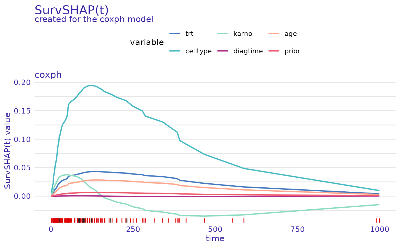
cph_predict_parts_survshap <- predict_parts(cph_exp, new_observation = veteran[1, -c(3, 4)])
head(cph_predict_parts_survshap$result)
#>               trt    celltype       karno      diagtime          age
#> t=1.5 0.001358479 0.005752629 0.002400785 -1.753141e-05 0.0007519409
#> t=4   0.003364680 0.014321361 0.005877960 -3.897254e-05 0.0018795538
#> t=7   0.005360141 0.022931960 0.009247829 -5.480637e-05 0.0030211319
#> t=8   0.007989085 0.034411531 0.013535810 -6.687523e-05 0.0045549833
#> t=10  0.009277550 0.040094562 0.015567469 -6.898441e-05 0.0053188972
#> t=12  0.011153127 0.048434497 0.018433696 -6.740775e-05 0.0064449115
#>              prior
#> t=1.5 0.0001596961
#> t=4   0.0004003893
#> t=7   0.0006457473
#> t=8   0.0009784720
#> t=10  0.0011456328
#> t=12  0.0013939562
plot(cph_predict_parts_survshap)


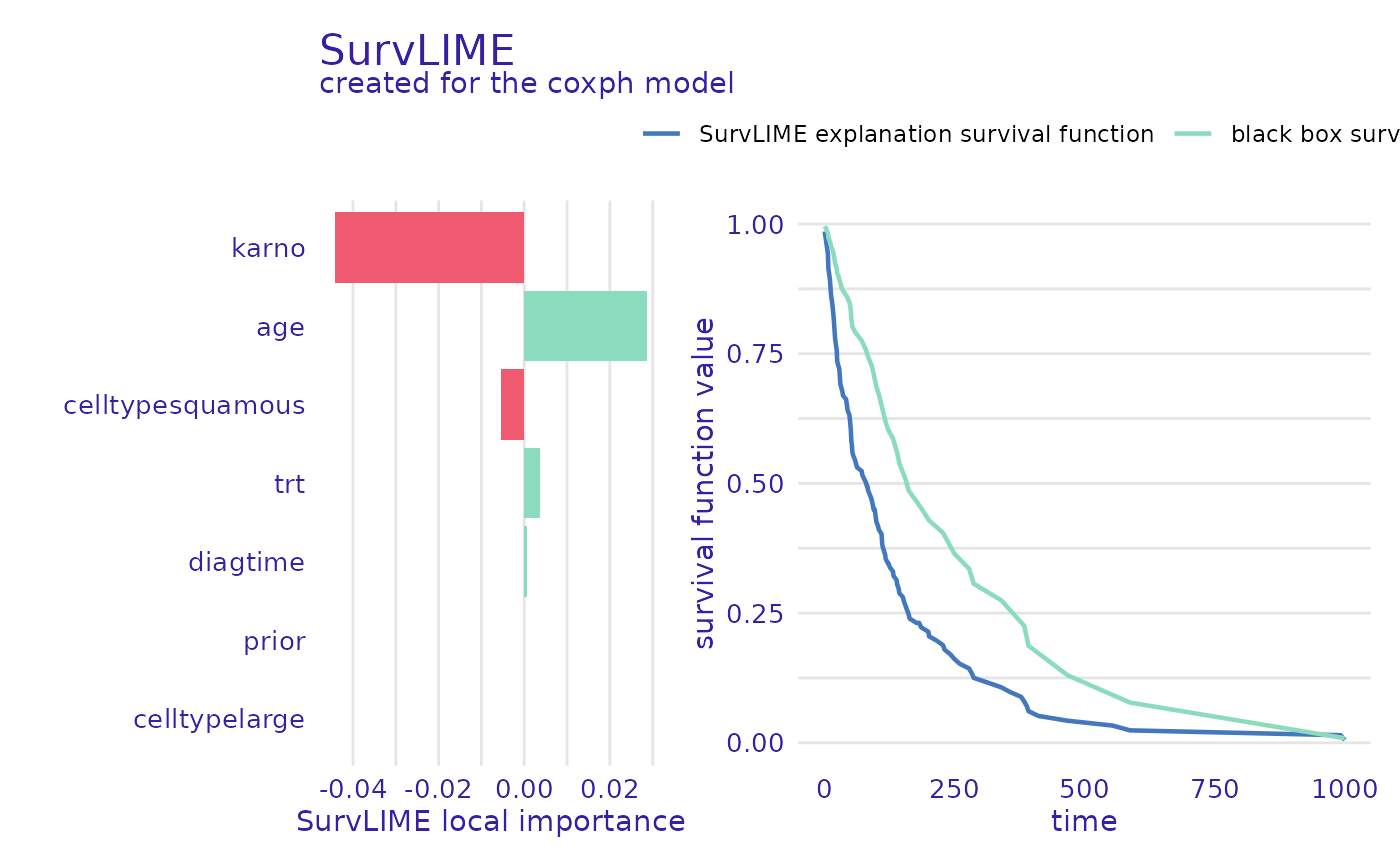
cph_predict_parts_survlime <- predict_parts(
    cph_exp,
    new_observation = veteran[1, -c(3, 4)],
    type = "survlime"
)
head(cph_predict_parts_survlime$result)
#>           trt         karno     diagtime          age       prior celltypelarge
#> 1 0.003629477 -0.0007383551 8.119279e-05 0.0004152425 0.000347701  -0.007316818
#>   celltypesmallcell celltypesquamous
#> 1       0.005774009     -0.005378658
plot(cph_predict_parts_survlime, type = "local_importance")

# }