Plot 2-Dimensional Model Profile for Survival Models
Source:R/plot_model_profile_2d.R
plot.model_profile_2d_survival.RdThis function plots objects of class "model_profile_2d_survival" created
using the model_profile_2d() function.
# S3 method for model_profile_2d_survival
plot(
  x,
  ...,
  variables = NULL,
  times = NULL,
  marginalize_over_time = FALSE,
  facet_ncol = NULL,
  title = "default",
  subtitle = "default",
  colors = NULL
)
Arguments
- x
an object of class
model_profile_2d_survivalto be plotted- ...
additional objects of class
model_profile_2d_survivalto be plotted together- variables
list of character vectors of length 2, names of pairs of variables to be plotted
- times
numeric vector, times for which the profile should be plotted, the times must be present in the 'times' field of the explainer. If
NULL(default) then the median survival time (if available) or the median time from the explainer object is used.- marginalize_over_time
logical, if
TRUEthen the profile is calculated for all times and then averaged over time, ifFALSE(default) then the profile is calculated for each time separately- facet_ncol
number of columns for arranging subplots
- title
character, title of the plot.
'default'automatically generates either "2D partial dependence survival profiles" or "2D accumulated local effects survival profiles" depending on the explanation type.- subtitle
character, subtitle of the plot,
'default'automatically generates "created for the XXX model", where XXX is the explainer labels, ifmarginalize_over_time = FALSE, time is also added to the subtitle- colors
character vector containing the colors to be used for plotting variables (containing either hex codes "#FF69B4", or names "blue")
Value
A collection of ggplot objects arranged with the patchwork package.
Examples
# \donttest{
library(survival)
library(survex)
cph <- coxph(Surv(time, status) ~ ., data = veteran, model = TRUE, x = TRUE, y = TRUE)
cph_exp <- explain(cph)
#> Preparation of a new explainer is initiated
#> -> model label : coxph ( default )
#> -> data : 137 rows 6 cols ( extracted from the model )
#> -> target variable : 137 values ( 128 events and 9 censored , censoring rate = 0.066 ) ( extracted from the model )
#> -> times : 50 unique time points , min = 1.5 , median survival time = 80 , max = 999
#> -> times : ( generated from y as uniformly distributed survival quantiles based on Kaplan-Meier estimator )
#> -> predict function : predict.coxph with type = 'risk' will be used ( default )
#> -> predict survival function : predictSurvProb.coxph will be used ( default )
#> -> predict cumulative hazard function : -log(predict_survival_function) will be used ( default )
#> -> model_info : package survival , ver. 3.7.0 , task survival ( default )
#> A new explainer has been created!
cph_model_profile_2d <- model_profile_2d(cph_exp,
variables = list(
c("age", "celltype"),
c("age", "karno")
)
)
head(cph_model_profile_2d$result)
#> _v1name_ _v2name_ _v1type_ _v2type_ _v1value_ _v2value_ _times_
#> 1 age celltype numerical categorical 34 adeno 1.5
#> 2 age celltype numerical categorical 35.9583333333333 adeno 1.5
#> 3 age celltype numerical categorical 37.9166666666667 adeno 1.5
#> 4 age celltype numerical categorical 39.875 adeno 1.5
#> 5 age celltype numerical categorical 41.8333333333333 adeno 1.5
#> 6 age celltype numerical categorical 43.7916666666667 adeno 1.5
#> _label_ _yhat_
#> 1 coxph 0.9711210
#> 2 coxph 0.9715980
#> 3 coxph 0.9720673
#> 4 coxph 0.9725290
#> 5 coxph 0.9729833
#> 6 coxph 0.9734302
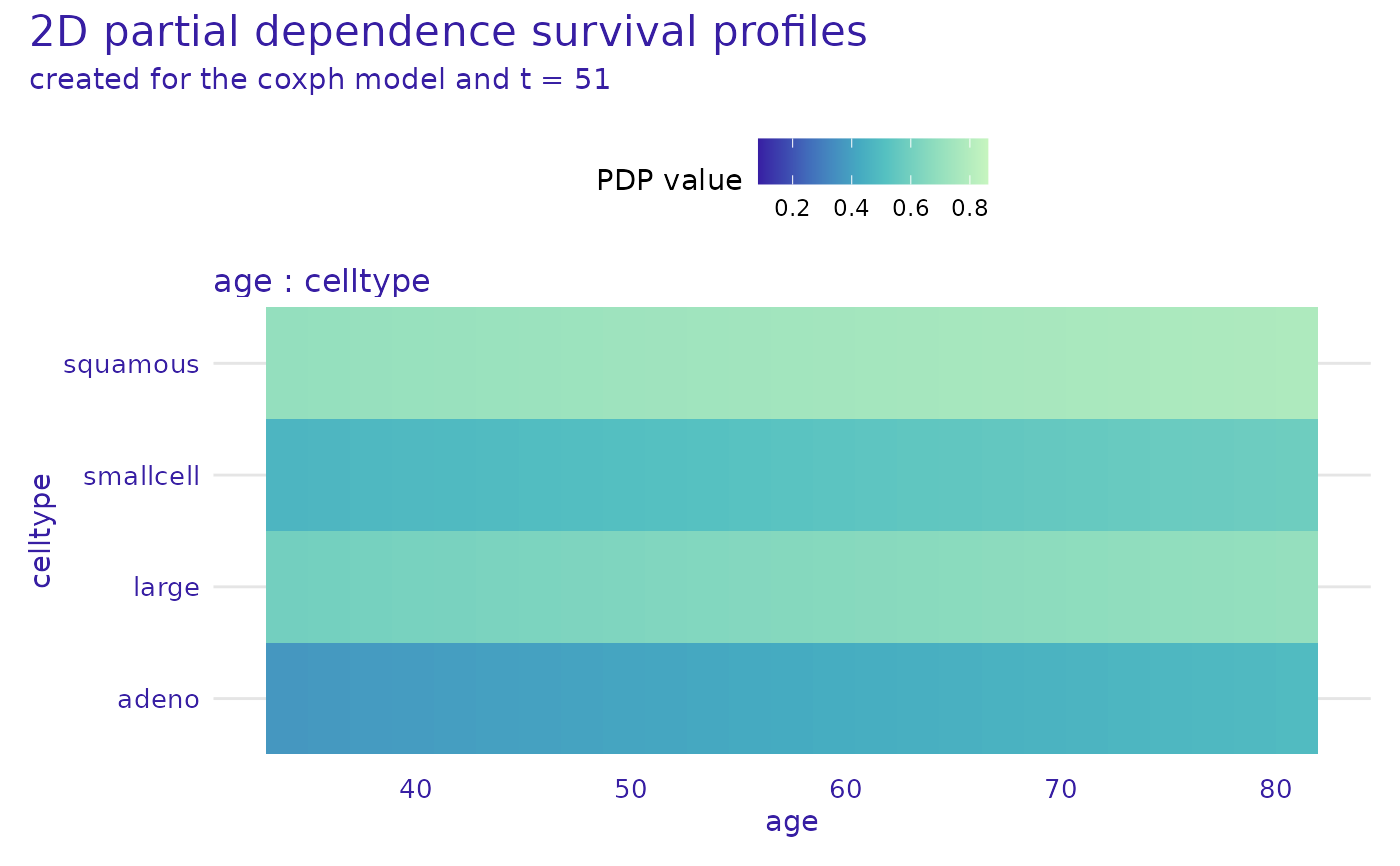
plot(cph_model_profile_2d, variables = list(c("age", "celltype")), times = cph_exp$times[20])
 cph_model_profile_2d_ale <- model_profile_2d(cph_exp,
variables = list(c("age", "karno")),
type = "accumulated"
)
head(cph_model_profile_2d_ale$result)
#> _v1name_ _v2name_ _v1type_ _v2type_ _v1value_ _v2value_ _times_ _yhat_
#> 1 age karno numerical numerical 34 10 1.5 0.9821661
#> 2 age karno numerical numerical 34 10 4.0 0.9562840
#> 3 age karno numerical numerical 34 10 7.0 0.9310471
#> 4 age karno numerical numerical 34 10 8.0 0.8984986
#> 5 age karno numerical numerical 34 10 10.0 0.8828059
#> 6 age karno numerical numerical 34 10 12.0 0.8602254
#> _right_ _left_ _top_ _bottom_ _count_ _label_
#> 1 36 34 10 15 0 coxph
#> 2 36 34 10 15 0 coxph
#> 3 36 34 10 15 0 coxph
#> 4 36 34 10 15 0 coxph
#> 5 36 34 10 15 0 coxph
#> 6 36 34 10 15 0 coxph
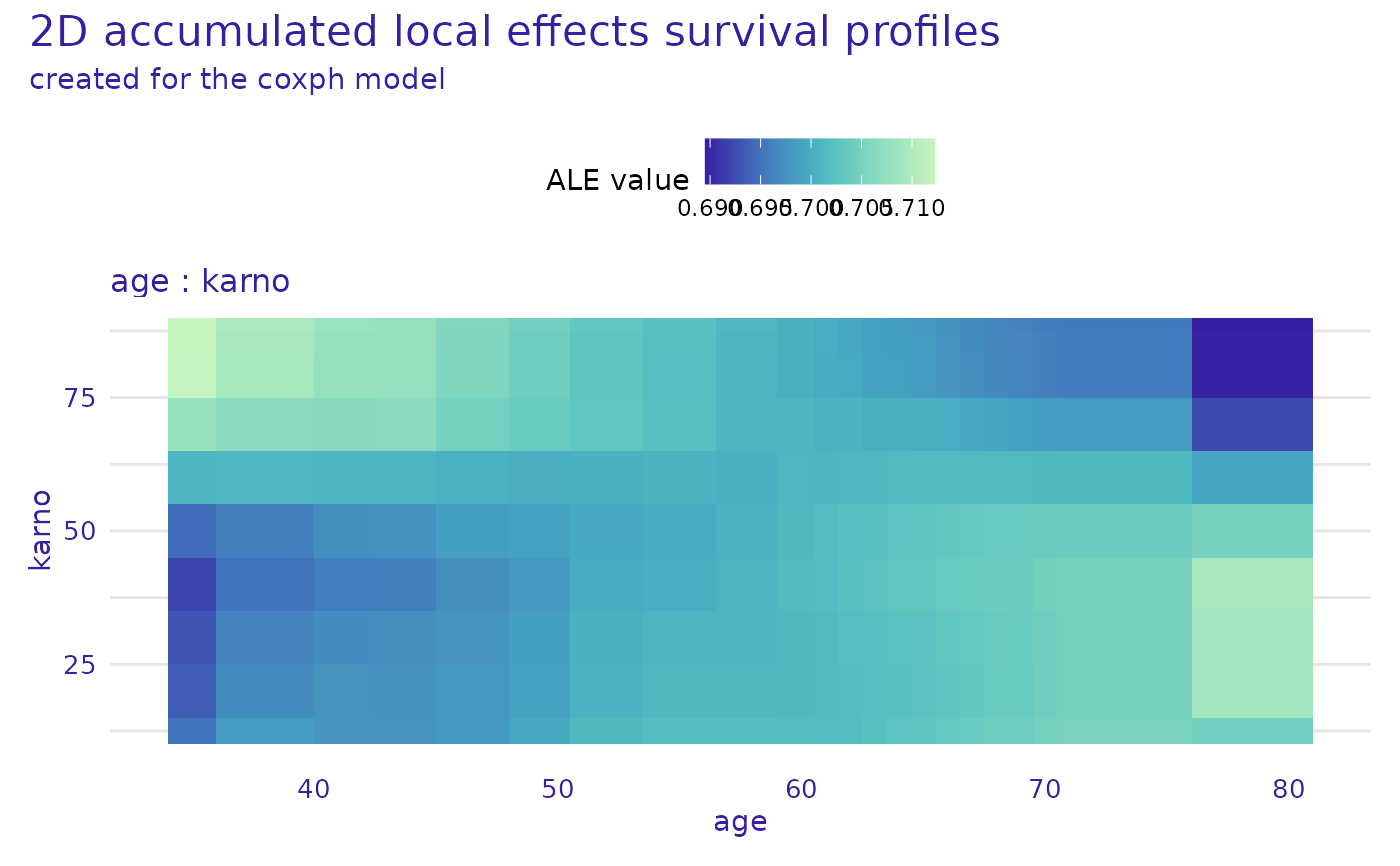
plot(cph_model_profile_2d_ale, times = cph_exp$times[c(10, 20)], marginalize_over_time = TRUE)
cph_model_profile_2d_ale <- model_profile_2d(cph_exp,
variables = list(c("age", "karno")),
type = "accumulated"
)
head(cph_model_profile_2d_ale$result)
#> _v1name_ _v2name_ _v1type_ _v2type_ _v1value_ _v2value_ _times_ _yhat_
#> 1 age karno numerical numerical 34 10 1.5 0.9821661
#> 2 age karno numerical numerical 34 10 4.0 0.9562840
#> 3 age karno numerical numerical 34 10 7.0 0.9310471
#> 4 age karno numerical numerical 34 10 8.0 0.8984986
#> 5 age karno numerical numerical 34 10 10.0 0.8828059
#> 6 age karno numerical numerical 34 10 12.0 0.8602254
#> _right_ _left_ _top_ _bottom_ _count_ _label_
#> 1 36 34 10 15 0 coxph
#> 2 36 34 10 15 0 coxph
#> 3 36 34 10 15 0 coxph
#> 4 36 34 10 15 0 coxph
#> 5 36 34 10 15 0 coxph
#> 6 36 34 10 15 0 coxph
plot(cph_model_profile_2d_ale, times = cph_exp$times[c(10, 20)], marginalize_over_time = TRUE)
 # }
# }