Regression example - apartments data • rSAFE

In this vignette we present an example of an application of the rSAFE package in case of regression problems. It is based on apartments and apartmentsTest datasets which come from the DALEX package but are also available in the rSAFE package. We will use these artificial datasets to predict the price per square meter of an apartment based on features such as construction year, surface, floor, number of rooms and district. It should be mentioned that four of these variables are continuous while the fifth one is categorical.

library(rSAFE)
head(apartments)
#>   m2.price construction.year surface floor no.rooms    district
#> 1     5897              1953      25     3        1 Srodmiescie
#> 2     1818              1992     143     9        5     Bielany
#> 3     3643              1937      56     1        2       Praga
#> 4     3517              1995      93     7        3      Ochota
#> 5     3013              1992     144     6        5     Mokotow
#> 6     5795              1926      61     6        2 Srodmiescie

Building a black-box model

First we fit a random forest model to the original apartments dataset - this is our complex model that will serve us as a surrogate.

library(randomForest)
set.seed(111)
model_rf1 <- randomForest(m2.price ~ construction.year + surface + floor + no.rooms + district, data = apartments)

Creating an explainer

We also create an explainer object that will be used later to create new variables and at the end to compare models performance.

library(DALEX)
explainer_rf1 <- explain(model_rf1, data = apartmentsTest[1:3000,2:6], y = apartmentsTest[1:3000,1], label = "rf1", verbose = FALSE)
explainer_rf1
#> Model label:  rf1 
#> Model class:  randomForest.formula,randomForest 
#> Data head  :
#>      construction.year surface floor no.rooms    district
#> 1001              1976     131     3        5 Srodmiescie
#> 1002              1978     112     9        4     Mokotow

Creating a safe_extractor

Now, we create a safe_extractor object using rSAFE package and our surrogate model. Setting the argument verbose=FALSE stops progress bar from printing.

safe_extractor <- safe_extraction(explainer_rf1, penalty = 25, verbose = FALSE)

Now, let’s print summary for the new object we have just created.

print(safe_extractor)
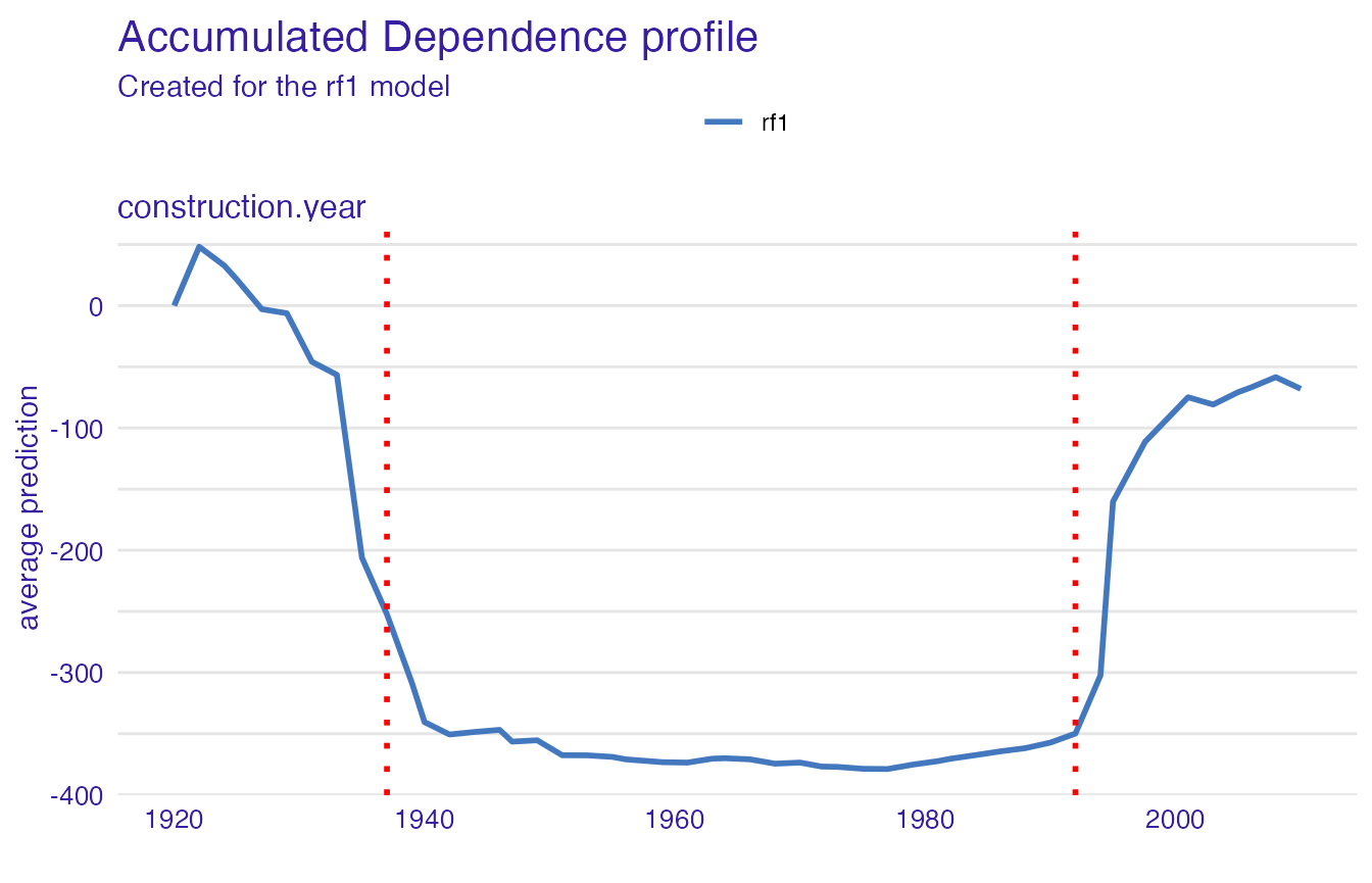
#> Variable 'construction.year' - selected intervals:
#>  (-Inf, 1937]
#>      (1937, 1992]
#>      (1992, Inf)
#> Variable 'surface' - selected intervals:
#>  (-Inf, 47]
#>      (47, 101]
#>      (101, Inf)
#> Variable 'floor' - selected intervals:
#>  (-Inf, 5]
#>      (5, Inf)
#> Variable 'no.rooms' - selected intervals:
#>  (-Inf, 3]
#>      (3, Inf)
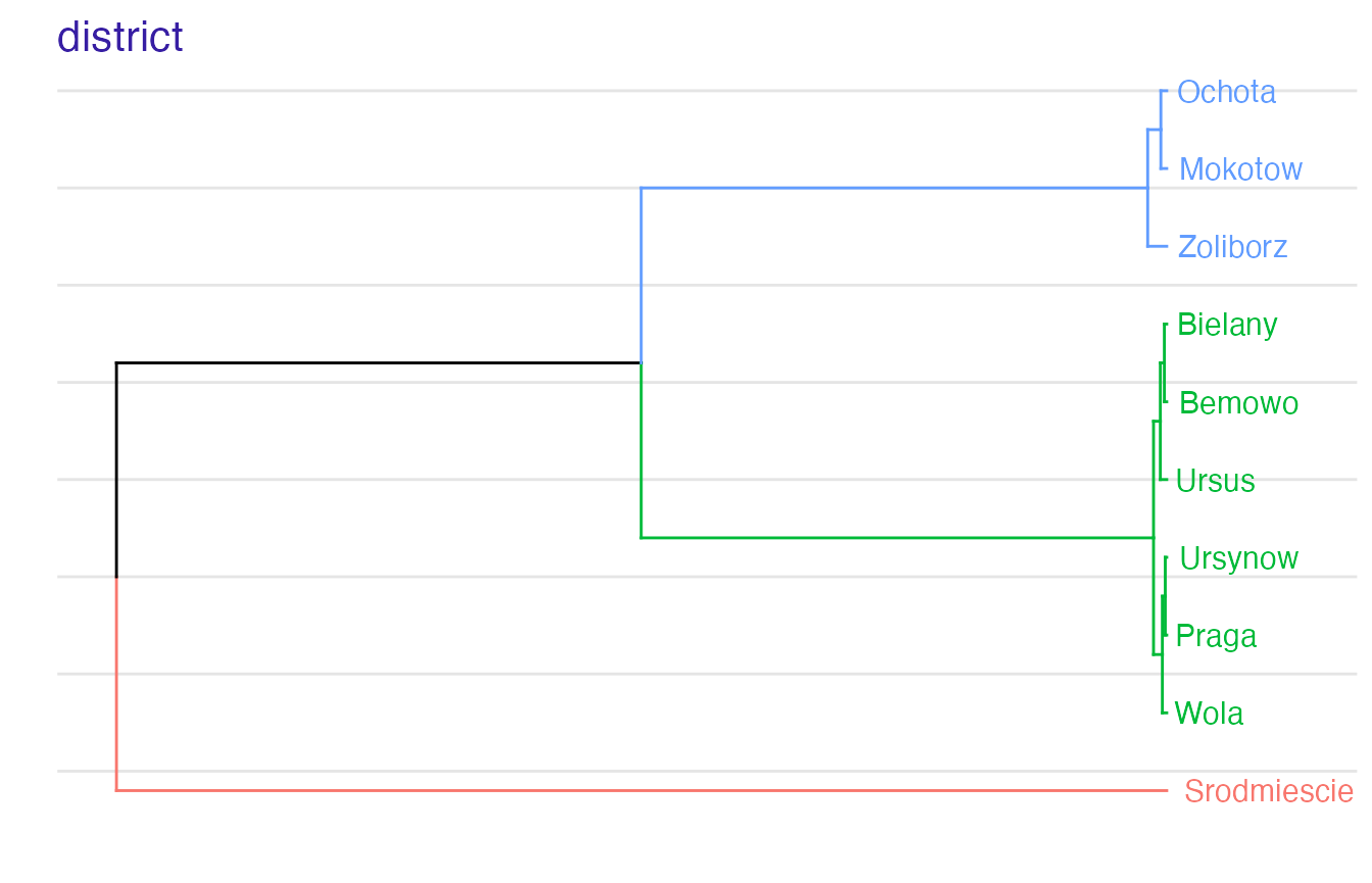
#> Variable 'district' - created levels:
#>  Bemowo, Bielany, Ursus, Ursynow, Praga, Wola ->  Bemowo_Bielany_Praga_Ursus_Ursynow_Wola 
#>  Zoliborz, Mokotow, Ochota ->  Mokotow_Ochota_Zoliborz 
#>  Srodmiescie ->  Srodmiescie

We can see transformation propositions for all variables in our dataset.

In the plot below we can see which points have been chosen to be the breakpoints for a particular variable:

plot(safe_extractor, variable = "construction.year")

For factor variables we can observe in which order levels have been merged and what is the optimal clustering:

plot(safe_extractor, variable = "district")

Transforming data

Now we can use our safe_extractor object to create new categorical features in the given dataset.

data1 <- safely_transform_data(safe_extractor, apartmentsTest[3001:6000,], verbose = FALSE)

district	m2.price	construction.year	surface	floor	no.rooms	construction.year_new	surface_new	floor_new	no.rooms_new	district_new
Bielany	3542	1979	21	6	1	(1937, 1992]	(-Inf, 47]	(5, Inf)	(-Inf, 3]	Bemowo_Bielany_Praga_Ursus_Ursynow_Wola
Srodmiescie	5631	1997	107	2	4	(1992, Inf)	(101, Inf)	(-Inf, 5]	(3, Inf)	Srodmiescie
Bielany	2989	1994	41	9	2	(1992, Inf)	(-Inf, 47]	(5, Inf)	(-Inf, 3]	Bemowo_Bielany_Praga_Ursus_Ursynow_Wola
Ursynow	3822	1968	28	2	2	(1937, 1992]	(-Inf, 47]	(-Inf, 5]	(-Inf, 3]	Bemowo_Bielany_Praga_Ursus_Ursynow_Wola
Ursynow	2337	1971	146	3	6	(1937, 1992]	(101, Inf)	(-Inf, 5]	(3, Inf)	Bemowo_Bielany_Praga_Ursus_Ursynow_Wola
Ochota	3381	1956	97	8	3	(1937, 1992]	(47, 101]	(5, Inf)	(-Inf, 3]	Mokotow_Ochota_Zoliborz

We can also perform feature selection if we wish. For each original feature it keeps exactly one of their forms - original one or transformed one.

vars <- safely_select_variables(safe_extractor, data1, which_y = "m2.price", verbose = FALSE)
data1 <- data1[,c("m2.price", vars)]
print(vars)
#> [1] "surface"               "floor"                 "no.rooms"             
#> [4] "construction.year_new" "district_new"

It can be observed that for some features the original form was preferred and for others the transformed one.

Here are the first few rows for our data after feature selection:

m2.price	surface	floor	no.rooms	construction.year_new	district_new
3542	21	6	1	(1937, 1992]	Bemowo_Bielany_Praga_Ursus_Ursynow_Wola
5631	107	2	4	(1992, Inf)	Srodmiescie
2989	41	9	2	(1992, Inf)	Bemowo_Bielany_Praga_Ursus_Ursynow_Wola
3822	28	2	2	(1937, 1992]	Bemowo_Bielany_Praga_Ursus_Ursynow_Wola
2337	146	3	6	(1937, 1992]	Bemowo_Bielany_Praga_Ursus_Ursynow_Wola
3381	97	8	3	(1937, 1992]	Mokotow_Ochota_Zoliborz

Now, we perform transformations on another data that will be used later in explainers.

data2 <- safely_transform_data(safe_extractor, apartmentsTest[6001:9000,], verbose = FALSE)[,c("m2.price", vars)]

Creating white-box models on original and transformed datasets

Let’s fit the models to data containing newly created columns. We consider a linear model as a white-box model.

model_lm2 <- lm(m2.price ~ ., data = data1)
explainer_lm2 <- explain(model_lm2, data = data2, y = apartmentsTest[6001:9000,1], label = "lm2", verbose = FALSE)
set.seed(111)
model_rf2 <- randomForest(m2.price ~ ., data = data1)
explainer_rf2 <- explain(model_rf2, data2, apartmentsTest[6001:9000,1], label = "rf2", verbose = FALSE)

Moreover, we create a linear model based on original apartments dataset and its corresponding explainer in order to check if our methodology improves results.

model_lm1 <- lm(m2.price ~ ., data = apartments)
explainer_lm1 <- explain(model_lm1, data = apartmentsTest[1:3000,2:6], y = apartmentsTest[1:3000,1], label = "lm1", verbose = FALSE)

Comparing models performance

Final step is the comparison of all the models we have created.

mp_lm1 <- model_performance(explainer_lm1)
mp_rf1 <- model_performance(explainer_rf1)
mp_lm2 <- model_performance(explainer_lm2)
mp_rf2 <- model_performance(explainer_rf2)

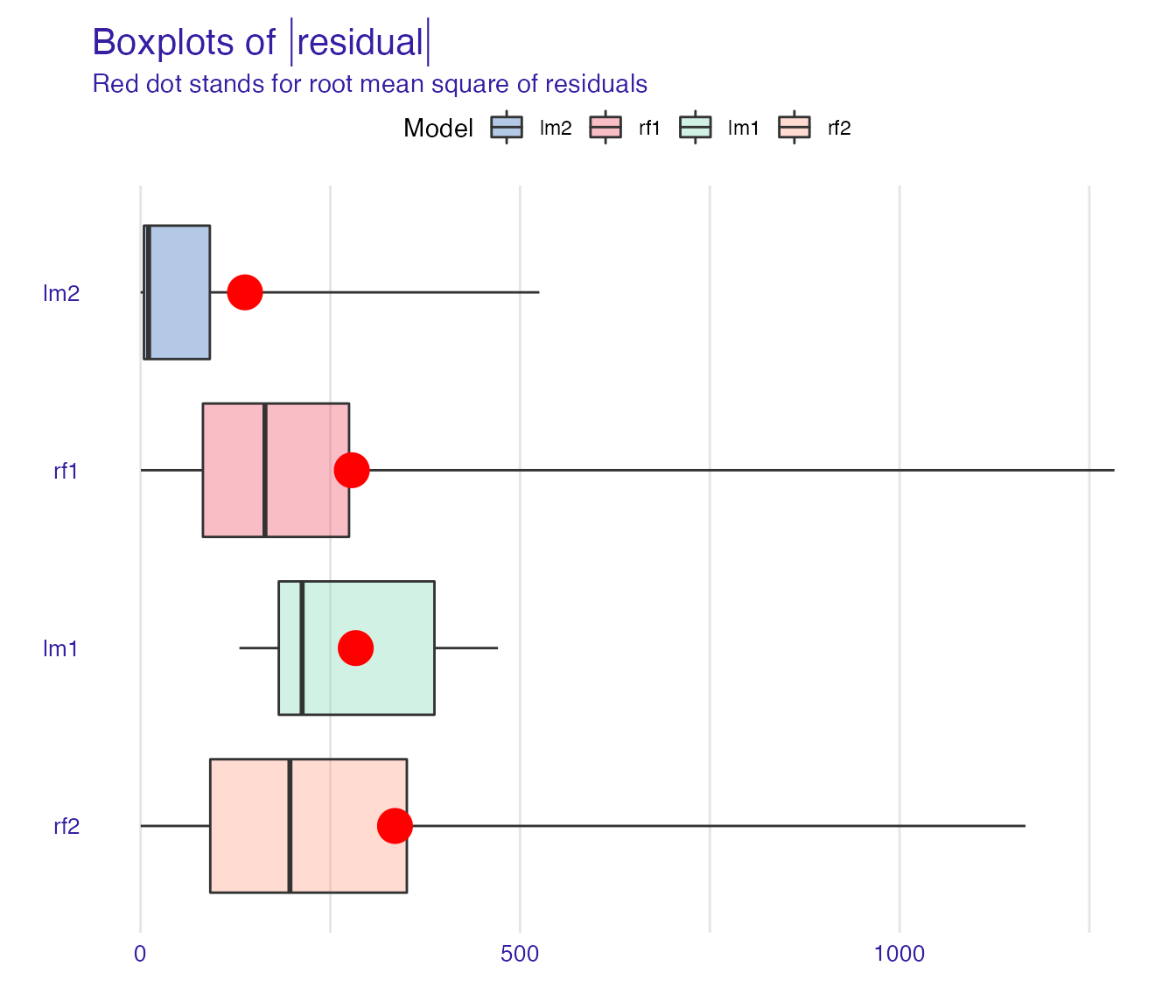
plot(mp_lm1, mp_rf1, mp_lm2, mp_rf2, geom = "boxplot")

In the plot above we can see that the linear model based on transformed features has generally more accurate predictions that the one fitted to the original dataset.

Regression example - apartments data