Introduction to localModel package

This vignette shows how localModel package can be used to explain regression models. We will use the apartments dataset from DALEX2 package. For more information about the dataset, please refer to the Gentle introduction to DALEX.

We will need localModel and DALEX2 packages. Random forest from randomForest package will serve as an example model, and linear regression as a simple model for comparison.

library(DALEX)
library(localModel)
library(randomForest)
data('apartments')
data('apartments_test')
set.seed(69)
mrf <- randomForest(m2.price ~., data = apartments, ntree = 50)
mlm <- lm(m2.price ~., data = apartments)

First, we need to create an explainer object, using the explain function. We will explain the prediction for fifth observation in the test dataset.

explainer <- DALEX::explain(model = mrf,
                     data = apartments_test[, -1])
#> Preparation of a new explainer is initiated
#>   -> model label       :  randomForest  ( [33m default [39m )
#>   -> data              :  9000  rows  5  cols 
#>   -> target variable   :  not specified! ( [31m WARNING [39m )
#>   -> predict function  :  yhat.randomForest  will be used ( [33m default [39m )
#>   -> predicted values  :  numerical, min =  1996.308 , mean =  3502.832 , max =  5666.4  
#>   -> model_info        :  package randomForest , ver. 4.6.14 , task regression ( [33m default [39m ) 
#>   -> residual function :  difference between y and yhat ( [33m default [39m )
#>  [32m A new explainer has been created! [39m
explainer2 <- DALEX::explain(model = mlm,
                      data = apartments_test[, -1])
#> Preparation of a new explainer is initiated
#>   -> model label       :  lm  ( [33m default [39m )
#>   -> data              :  9000  rows  5  cols 
#>   -> target variable   :  not specified! ( [31m WARNING [39m )
#>   -> predict function  :  yhat.lm  will be used ( [33m default [39m )
#>   -> predicted values  :  numerical, min =  1792.597 , mean =  3506.836 , max =  6241.447  
#>   -> model_info        :  package stats , ver. 4.0.2 , task regression ( [33m default [39m ) 
#>   -> residual function :  difference between y and yhat ( [33m default [39m )
#>  [32m A new explainer has been created! [39m
new_observation <- apartments_test[5, -1]
new_observation
#>      construction.year surface floor no.rooms district
#> 1005              1978     102     4        4   Bemowo

Local explanation is created via individual_surrogate_model function, which takes the explainer, observation of interest and number of new observations to simulate as argument. Optionally, we can set seed using the seed parameter for reproducibility.

model_lok <- individual_surrogate_model(explainer, new_observation,
                                        size = 500, seed = 17)
model_lok2 <- individual_surrogate_model(explainer2, new_observation,
                                         size = 500, seed = 17)

First, local interpretable features are created. Numerical features are discretized by using decision tree to model relationship between the feature and the corresponding Ceteris Paribus profile. Categorical features are also discretized by merging levels using the marginal relationship between the feature and the model response. Then, new dataset is simulated by switching a random number of interpretable inputs in the explained instance. This procedure mimics “graying out” areas (superpixels) in the original LIME method. LASSO regression model is fitted to the model response for these new observations, which makes the final explanations sparse and thus readable. More details can be found in the Methodology behind localModel package vignette.

The explanation can be plotted using generic plot function. The plot shows interpretable features and weights associated with them, starting at the model intercept. Negative weights are associated with features that decrease the apartment price, while positive weights increase it. We can plot explanation for two or more models together by passing several local explainer to plot function.

plot(model_lok, model_lok2)

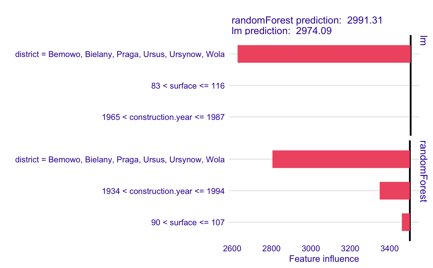
We can see that for this observation, the price predicted by Random Forest is negatively influeced mostly by the district and construction year, while linear regression ignores the effect of construction year.

Mateusz Staniak