This function calculates ceteris paribus profiles for grid of values spanned by two variables. It may be useful to identify or present interactions between two variables.
ceteris_paribus_2d(explainer, observation, grid_points = 101, variables = NULL)Arguments
- explainer
a model to be explained, preprocessed by the
DALEX::explain()function- observation
a new observation for which predictions need to be explained
- grid_points
number of points used for response path. Will be used for both variables
- variables
if specified, then only these variables will be explained
Value
an object of the class ceteris_paribus_2d_explainer.
References
Explanatory Model Analysis. Explore, Explain, and Examine Predictive Models. https://ema.drwhy.ai/
Examples
library("DALEX")
library("ingredients")
model_titanic_glm <- glm(survived ~ age + fare,
data = titanic_imputed, family = "binomial")
# \donttest{
explain_titanic_glm <- explain(model_titanic_glm,
data = titanic_imputed[,-8],
y = titanic_imputed[,8])
#> Preparation of a new explainer is initiated
#> -> model label : lm ( default )
#> -> data : 2207 rows 7 cols
#> -> target variable : 2207 values
#> -> predict function : yhat.glm will be used ( default )
#> -> predicted values : No value for predict function target column. ( default )
#> -> model_info : package stats , ver. 4.2.2 , task classification ( default )
#> -> predicted values : numerical, min = 0.1707237 , mean = 0.3221568 , max = 0.9983551
#> -> residual function : difference between y and yhat ( default )
#> -> residuals : numerical, min = -0.9519492 , mean = 4.78827e-11 , max = 0.8167072
#> A new explainer has been created!
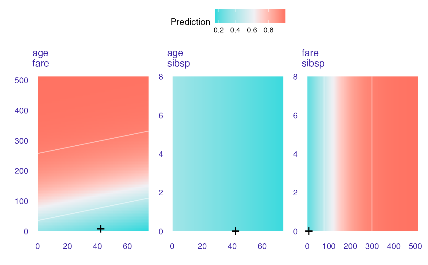
cp_rf <- ceteris_paribus_2d(explain_titanic_glm, titanic_imputed[1,],
variables = c("age", "fare", "sibsp"))
head(cp_rf)
#> y_hat new_x1 new_x2 vname1 vname2 label
#> 1 0.3545941 0.1666667 0.000000 age fare lm
#> 1.1 0.3719860 0.1666667 5.120607 age fare lm
#> 1.2 0.3897159 0.1666667 10.241214 age fare lm
#> 1.3 0.4077422 0.1666667 15.361821 age fare lm
#> 1.4 0.4260202 0.1666667 20.482428 age fare lm
#> 1.5 0.4445026 0.1666667 25.603035 age fare lm
plot(cp_rf)
#> Warning: The following aesthetics were dropped during statistical transformation: fill
#> ℹ This can happen when ggplot fails to infer the correct grouping structure in
#> the data.
#> ℹ Did you forget to specify a `group` aesthetic or to convert a numerical
#> variable into a factor?
#> Warning: `stat_contour()`: Zero contours were generated
#> Warning: no non-missing arguments to min; returning Inf
#> Warning: no non-missing arguments to max; returning -Inf
#> Warning: The following aesthetics were dropped during statistical transformation: fill
#> ℹ This can happen when ggplot fails to infer the correct grouping structure in
#> the data.
#> ℹ Did you forget to specify a `group` aesthetic or to convert a numerical
#> variable into a factor?
#> Warning: Raster pixels are placed at uneven horizontal intervals and will be shifted
#> ℹ Consider using `geom_tile()` instead.
#> Warning: Raster pixels are placed at uneven horizontal intervals and will be shifted
#> ℹ Consider using `geom_tile()` instead.
 library("ranger")
set.seed(59)
apartments_rf_model <- ranger(m2.price ~., data = apartments)
explainer_rf <- explain(apartments_rf_model,
data = apartments_test[,-1],
y = apartments_test[,1],
label = "ranger forest",
verbose = FALSE)
new_apartment <- apartments_test[1,]
new_apartment
#> m2.price construction.year surface floor no.rooms district
#> 1001 4644 1976 131 3 5 Srodmiescie
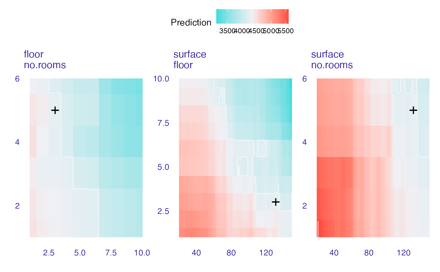
wi_rf_2d <- ceteris_paribus_2d(explainer_rf, observation = new_apartment,
variables = c("surface", "floor", "no.rooms"))
head(wi_rf_2d)
#> y_hat new_x1 new_x2 vname1 vname2 label
#> 1 5130.866 20 1.00 surface floor ranger forest
#> 2 5130.866 20 1.09 surface floor ranger forest
#> 3 5130.866 20 1.18 surface floor ranger forest
#> 4 5130.866 20 1.27 surface floor ranger forest
#> 5 5130.866 20 1.36 surface floor ranger forest
#> 6 5130.866 20 1.45 surface floor ranger forest
plot(wi_rf_2d)
#> Warning: The following aesthetics were dropped during statistical transformation: fill
#> ℹ This can happen when ggplot fails to infer the correct grouping structure in
#> the data.
#> ℹ Did you forget to specify a `group` aesthetic or to convert a numerical
#> variable into a factor?
#> Warning: The following aesthetics were dropped during statistical transformation: fill
#> ℹ This can happen when ggplot fails to infer the correct grouping structure in
#> the data.
#> ℹ Did you forget to specify a `group` aesthetic or to convert a numerical
#> variable into a factor?
#> Warning: The following aesthetics were dropped during statistical transformation: fill
#> ℹ This can happen when ggplot fails to infer the correct grouping structure in
#> the data.
#> ℹ Did you forget to specify a `group` aesthetic or to convert a numerical
#> variable into a factor?
#> Warning: Raster pixels are placed at uneven horizontal intervals and will be shifted
#> ℹ Consider using `geom_tile()` instead.
#> Warning: Raster pixels are placed at uneven horizontal intervals and will be shifted
#> ℹ Consider using `geom_tile()` instead.
library("ranger")
set.seed(59)
apartments_rf_model <- ranger(m2.price ~., data = apartments)
explainer_rf <- explain(apartments_rf_model,
data = apartments_test[,-1],
y = apartments_test[,1],
label = "ranger forest",
verbose = FALSE)
new_apartment <- apartments_test[1,]
new_apartment
#> m2.price construction.year surface floor no.rooms district
#> 1001 4644 1976 131 3 5 Srodmiescie
wi_rf_2d <- ceteris_paribus_2d(explainer_rf, observation = new_apartment,
variables = c("surface", "floor", "no.rooms"))
head(wi_rf_2d)
#> y_hat new_x1 new_x2 vname1 vname2 label
#> 1 5130.866 20 1.00 surface floor ranger forest
#> 2 5130.866 20 1.09 surface floor ranger forest
#> 3 5130.866 20 1.18 surface floor ranger forest
#> 4 5130.866 20 1.27 surface floor ranger forest
#> 5 5130.866 20 1.36 surface floor ranger forest
#> 6 5130.866 20 1.45 surface floor ranger forest
plot(wi_rf_2d)
#> Warning: The following aesthetics were dropped during statistical transformation: fill
#> ℹ This can happen when ggplot fails to infer the correct grouping structure in
#> the data.
#> ℹ Did you forget to specify a `group` aesthetic or to convert a numerical
#> variable into a factor?
#> Warning: The following aesthetics were dropped during statistical transformation: fill
#> ℹ This can happen when ggplot fails to infer the correct grouping structure in
#> the data.
#> ℹ Did you forget to specify a `group` aesthetic or to convert a numerical
#> variable into a factor?
#> Warning: The following aesthetics were dropped during statistical transformation: fill
#> ℹ This can happen when ggplot fails to infer the correct grouping structure in
#> the data.
#> ℹ Did you forget to specify a `group` aesthetic or to convert a numerical
#> variable into a factor?
#> Warning: Raster pixels are placed at uneven horizontal intervals and will be shifted
#> ℹ Consider using `geom_tile()` instead.
#> Warning: Raster pixels are placed at uneven horizontal intervals and will be shifted
#> ℹ Consider using `geom_tile()` instead.
 # }
# }