Dataset Level Performance Measures
Source:R/model_performance.R
model_performance.surv_explainer.RdThis function calculates metrics for survival models. The metrics calculated are C/D AUC, Brier score, and their integrated versions, as well as concordance index. It also can calculate ROC curves for specific selected time points.
model_performance(explainer, ...)

# S3 method for surv_explainer
model_performance(
  explainer,
  ...,
  type = "metrics",
  metrics = c(`C-index` = c_index, `Integrated C/D AUC` = integrated_cd_auc,
    `Brier score` = brier_score, `Integrated Brier score` = integrated_brier_score,
    `C/D AUC` = cd_auc),
  times = NULL
)
Arguments
- explainer
an explainer object - model preprocessed by the
explain()function- ...
other parameters, currently ignored
- type
character, either
"metrics"or"roc". If"metrics"then performance metrics are calculated, if"roc"ROC curves for selected time points are calculated.- metrics
a named vector containing the metrics to be calculated. The values should be standardized loss functions. The functions can be supplied manually but has to have these named parameters (
y_true,risk,surv,times), wherey_truerepresents thesurvival::Survobject with observed times and statuses,riskis the risk score calculated by the model, andsurvis the survival function for each observation evaluated attimes.- times
a numeric vector of times. If
type == "metrics"then the survival function is evaluated at these times, iftype == "roc"then the ROC curves are calculated at these times.
Value
An object of class "model_performance_survival". It's a list of metric values calculated for the model. It contains:
Harrell's concordance index [1]
Brier score [2, 3]
C/D AUC using the estimator proposed by Uno et. al [4]
integral of the Brier score
integral of the C/D AUC
References
[1] Harrell, F.E., Jr., et al. "Regression modelling strategies for improved prognostic prediction." Statistics in Medicine 3.2 (1984): 143-152.
[2] Brier, Glenn W. "Verification of forecasts expressed in terms of probability." Monthly Weather Review 78.1 (1950): 1-3.
[3] Graf, Erika, et al. "Assessment and comparison of prognostic classification schemes for survival data." Statistics in Medicine 18.17‐18 (1999): 2529-2545.
[4] Uno, Hajime, et al. "Evaluating prediction rules for t-year survivors with censored regression models." Journal of the American Statistical Association 102.478 (2007): 527-537.
Examples
# \donttest{
library(survival)
library(survex)
cph <- coxph(Surv(time, status) ~ ., data = veteran, model = TRUE, x = TRUE, y = TRUE)
rsf_ranger <- ranger::ranger(Surv(time, status) ~ .,
data = veteran,
respect.unordered.factors = TRUE,
num.trees = 100,
mtry = 3,
max.depth = 5
)
rsf_src <- randomForestSRC::rfsrc(Surv(time, status) ~ .,
data = veteran
)
cph_exp <- explain(cph)
#> Preparation of a new explainer is initiated
#> -> model label : coxph ( default )
#> -> data : 137 rows 6 cols ( extracted from the model )
#> -> target variable : 137 values ( 128 events and 9 censored , censoring rate = 0.066 ) ( extracted from the model )
#> -> times : 50 unique time points , min = 1.5 , median survival time = 80 , max = 999
#> -> times : ( generated from y as uniformly distributed survival quantiles based on Kaplan-Meier estimator )
#> -> predict function : predict.coxph with type = 'risk' will be used ( default )
#> -> predict survival function : predictSurvProb.coxph will be used ( default )
#> -> predict cumulative hazard function : -log(predict_survival_function) will be used ( default )
#> -> model_info : package survival , ver. 3.7.0 , task survival ( default )
#> A new explainer has been created!
rsf_ranger_exp <- explain(rsf_ranger,
data = veteran[, -c(3, 4)],
y = Surv(veteran$time, veteran$status)
)
#> Preparation of a new explainer is initiated
#> -> model label : ranger ( default )
#> -> data : 137 rows 6 cols
#> -> target variable : 137 values ( 128 events and 9 censored )
#> -> times : 50 unique time points , min = 1.5 , median survival time = 80 , max = 999
#> -> times : ( generated from y as uniformly distributed survival quantiles based on Kaplan-Meier estimator )
#> -> predict function : sum over the predict_cumulative_hazard_function will be used ( default )
#> -> predict survival function : stepfun based on predict.ranger()$survival will be used ( default )
#> -> predict cumulative hazard function : stepfun based on predict.ranger()$chf will be used ( default )
#> -> model_info : package ranger , ver. 0.16.0 , task survival ( default )
#> A new explainer has been created!
rsf_src_exp <- explain(rsf_src)
#> Preparation of a new explainer is initiated
#> -> model label : rfsrc ( default )
#> -> data : 137 rows 6 cols ( extracted from the model )
#> -> target variable : 137 values ( 128 events and 9 censored , censoring rate = 0.066 ) ( extracted from the model )
#> -> times : 50 unique time points , min = 1.5 , median survival time = 80 , max = 999
#> -> times : ( generated from y as uniformly distributed survival quantiles based on Kaplan-Meier estimator )
#> -> predict function : sum over the predict_cumulative_hazard_function will be used ( default )
#> -> predict survival function : stepfun based on predict.rfsrc()$survival will be used ( default )
#> -> predict cumulative hazard function : stepfun based on predict.rfsrc()$chf will be used ( default )
#> -> model_info : package randomForestSRC , ver. 3.2.3 , task survival ( default )
#> A new explainer has been created!
cph_model_performance <- model_performance(cph_exp)
rsf_ranger_model_performance <- model_performance(rsf_ranger_exp)
rsf_src_model_performance <- model_performance(rsf_src_exp)
print(cph_model_performance)
#> $result
#> $result$`C-index`
#> [1] 0.7360464
#> attr(,"loss_type")
#> [1] "risk-based"
#>
#> $result$`Integrated C/D AUC`
#> [1] 0.8105198
#> attr(,"loss_type")
#> [1] "integrated"
#>
#> $result$`Brier score`
#> [1] 0.014504694 0.033959034 0.050857211 0.072372854 0.082965051 0.100349471
#> [7] 0.108958586 0.121159215 0.125346710 0.128121958 0.128948438 0.134527428
#> [13] 0.138530900 0.142016610 0.150285473 0.158946515 0.158878661 0.171125620
#> [19] 0.157656684 0.153866264 0.155959101 0.164717177 0.163641669 0.167682707
#> [25] 0.156722788 0.158009982 0.151887243 0.151107331 0.152375352 0.157368703
#> [31] 0.164691632 0.167253185 0.170942290 0.165724502 0.160732066 0.159359669
#> [37] 0.148453543 0.146427436 0.136663232 0.135249898 0.125593998 0.107657944
#> [43] 0.099012796 0.090316700 0.077607024 0.057225102 0.045652900 0.036427095
#> [49] 0.017892650 0.000299962
#> attr(,"loss_type")
#> [1] "time-dependent"
#>
#> $result$`Integrated Brier score`
#> [1] 0.0574109
#> attr(,"loss_type")
#> [1] "integrated"
#>
#> $result$`C/D AUC`
#> [1] 0.6592593 0.8045455 0.8352713 0.7846667 0.7845528 0.7411765 0.7506690
#> [8] 0.7628458 0.7982143 0.8151515 0.8487523 0.8512279 0.8333333 0.8296703
#> [15] 0.8165414 0.8084541 0.8184397 0.7926437 0.8245732 0.8392857 0.8405041
#> [22] 0.8230108 0.8264127 0.8191898 0.8432836 0.8375428 0.8454545 0.8485378
#> [29] 0.8353549 0.8234483 0.8033097 0.7910557 0.7764411 0.7830979 0.7830033
#> [36] 0.7801256 0.7964090 0.7876756 0.7825000 0.7643021 0.7701149 0.7852941
#> [43] 0.7775956 0.7816377 0.7849928 0.8149225 0.8689567 0.8120301 0.8740741
#> [50] NaN
#> attr(,"loss_type")
#> [1] "time-dependent"
#>
#>
#> $eval_times
#> [1] 1.5 4.0 7.0 8.0 10.0 12.0 13.0 16.0 18.0 19.0 21.0 24.0
#> [13] 25.0 27.0 30.0 33.0 36.0 44.0 49.0 51.0 52.0 54.0 59.0 72.0
#> [25] 80.0 84.0 92.0 95.0 100.0 105.0 111.0 117.0 122.0 132.0 140.0 144.0
#> [37] 156.0 162.0 186.0 201.0 228.0 250.0 278.0 287.0 340.0 384.0 392.0 467.0
#> [49] 587.0 999.0
#>
#> $event_times
#> 1 2 3 4 5 6 7 8 9 10 11 12 13 14 15 16 17 18 19 20
#> 72 411 228 126 118 10 82 110 314 100 42 8 144 25 11 30 384 4 54 13
#> 21 22 23 24 25 26 27 28 29 30 31 32 33 34 35 36 37 38 39 40
#> 123 97 153 59 117 16 151 22 56 21 18 139 20 31 52 287 18 51 122 27
#> 41 42 43 44 45 46 47 48 49 50 51 52 53 54 55 56 57 58 59 60
#> 54 7 63 392 10 8 92 35 117 132 12 162 3 95 177 162 216 553 278 12
#> 61 62 63 64 65 66 67 68 69 70 71 72 73 74 75 76 77 78 79 80
#> 260 200 156 182 143 105 103 250 100 999 112 87 231 242 991 111 1 587 389 33
#> 81 82 83 84 85 86 87 88 89 90 91 92 93 94 95 96 97 98 99 100
#> 25 357 467 201 1 30 44 283 15 25 103 21 13 87 2 20 7 24 99 8
#> 101 102 103 104 105 106 107 108 109 110 111 112 113 114 115 116 117 118 119 120
#> 99 61 25 95 80 51 29 24 18 83 31 51 90 52 73 8 36 48 7 140
#> 121 122 123 124 125 126 127 128 129 130 131 132 133 134 135 136 137
#> 186 84 19 45 80 52 164 19 53 15 43 340 133 111 231 378 49
#>
#> $event_statuses
#> 1 2 3 4 5 6 7 8 9 10 11 12 13 14 15 16 17 18 19 20
#> 1 1 1 1 1 1 1 1 1 0 1 1 1 0 1 1 1 1 1 1
#> 21 22 23 24 25 26 27 28 29 30 31 32 33 34 35 36 37 38 39 40
#> 0 0 1 1 1 1 1 1 1 1 1 1 1 1 1 1 1 1 1 1
#> 41 42 43 44 45 46 47 48 49 50 51 52 53 54 55 56 57 58 59 60
#> 1 1 1 1 1 1 1 1 1 1 1 1 1 1 1 1 1 1 1 1
#> 61 62 63 64 65 66 67 68 69 70 71 72 73 74 75 76 77 78 79 80
#> 1 1 1 0 1 1 1 1 1 1 1 0 0 1 1 1 1 1 1 1
#> 81 82 83 84 85 86 87 88 89 90 91 92 93 94 95 96 97 98 99 100
#> 1 1 1 1 1 1 1 1 1 1 0 1 1 1 1 1 1 1 1 1
#> 101 102 103 104 105 106 107 108 109 110 111 112 113 114 115 116 117 118 119 120
#> 1 1 1 1 1 1 1 1 1 0 1 1 1 1 1 1 1 1 1 1
#> 121 122 123 124 125 126 127 128 129 130 131 132 133 134 135 136 137
#> 1 1 1 1 1 1 1 1 1 1 1 1 1 1 1 1 1
#>
#> attr(,"class")
#> [1] "model_performance_survival" "surv_model_performance"
#> [3] "list"
#> attr(,"label")
#> [1] "coxph"
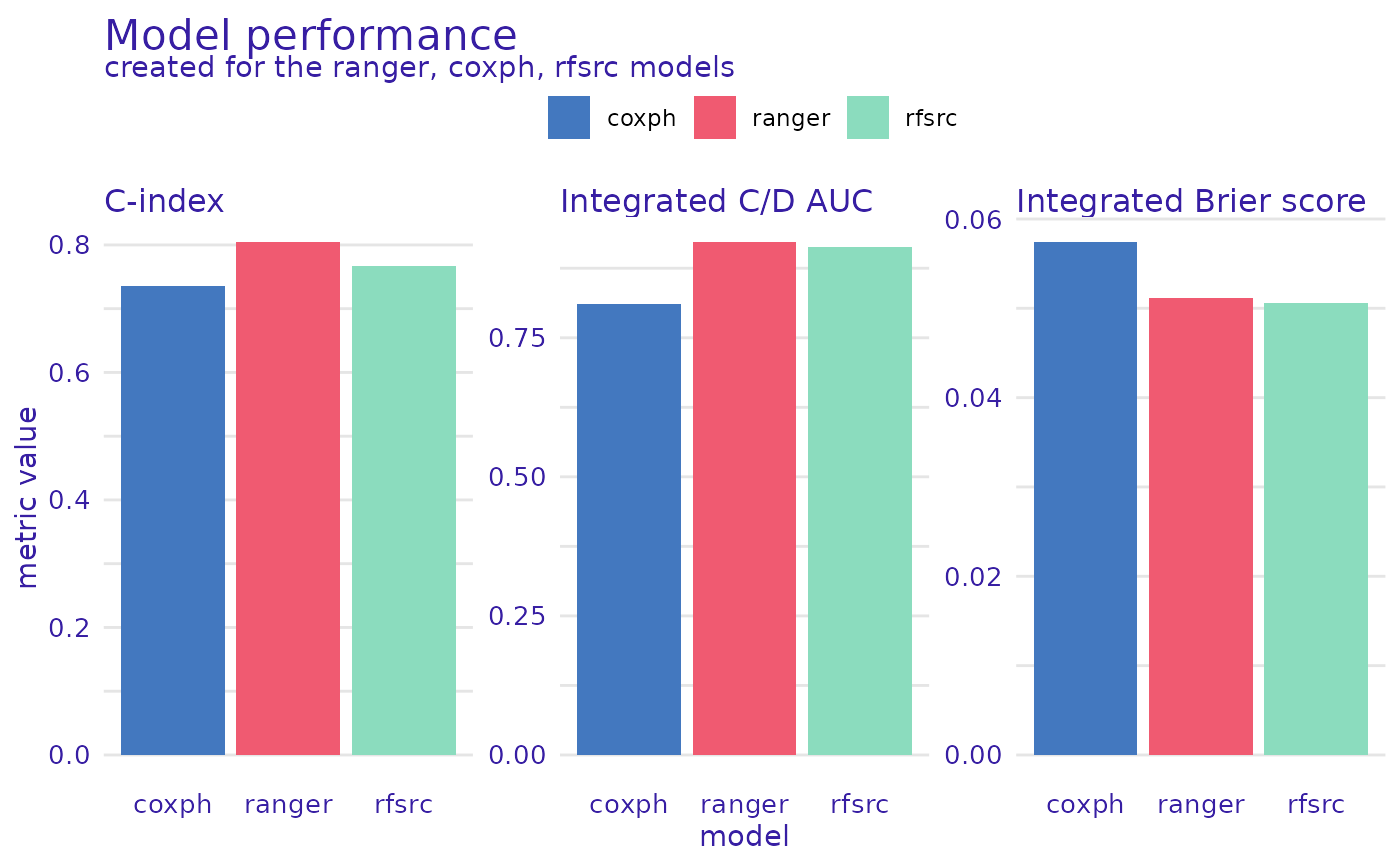
plot(rsf_ranger_model_performance, cph_model_performance,
rsf_src_model_performance,
metrics_type = "scalar"
)
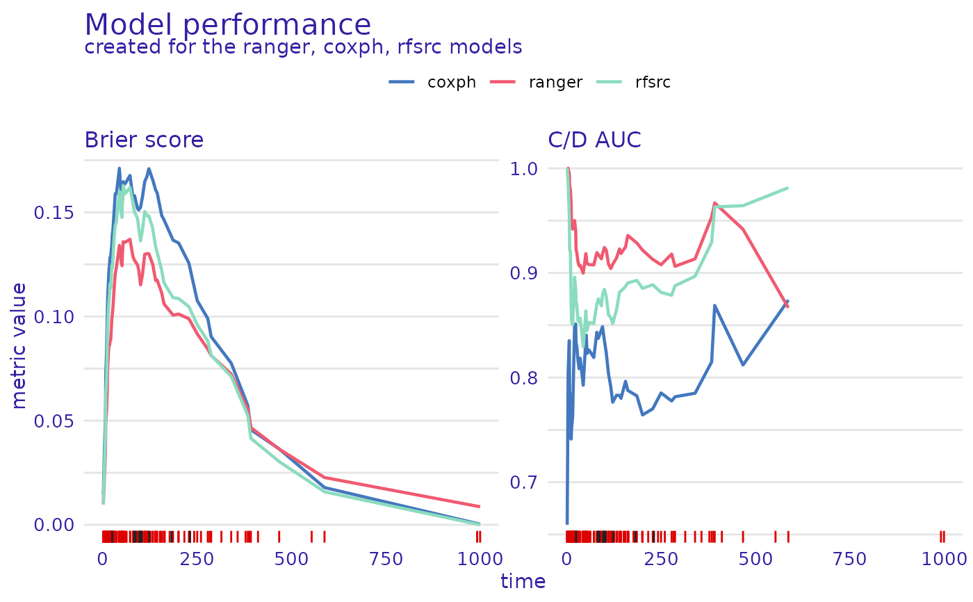
 plot(rsf_ranger_model_performance, cph_model_performance, rsf_src_model_performance)
#> Warning: Removed 3 rows containing missing values or values outside the scale range
#> (`geom_line()`).
plot(rsf_ranger_model_performance, cph_model_performance, rsf_src_model_performance)
#> Warning: Removed 3 rows containing missing values or values outside the scale range
#> (`geom_line()`).
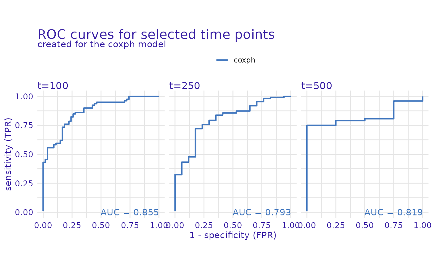
 cph_model_performance_roc <- model_performance(cph_exp, type = "roc", times = c(100, 250, 500))
plot(cph_model_performance_roc)
cph_model_performance_roc <- model_performance(cph_exp, type = "roc", times = c(100, 250, 500))
plot(cph_model_performance_roc)
 # }
# }