Plots Attributions for Variables of Individual Prediction

Function 'plot.individual_variable_effect' plots variables effects plots.

# S3 method for individual_variable_effect
plot(
  x,
  ...,
  id = 1,
  digits = 2,
  rounding_function = round,
  show_predicted = TRUE,
  show_attributions = TRUE,
  cols = c("label", "id"),
  rows = "ylevel",
  selected = NULL,
  bar_width = 8,
  vcolors = c(`-` = "#f05a71", `0` = "#371ea3", `+` = "#8bdcbe", X = "#371ea3", pred =
    "#371ea3")
)

Arguments

x	an individual variable effect explainer produced with function `individual_variable_effect()`
...	other explainers that shall be plotted together
id	of observation. By default first observation is taken.
digits	number of decimal places (round) or significant digits (signif) to be used. See the rounding_function argument.
rounding_function	function that is to used for rounding numbers. It may be signif() which keeps a specified number of significant digits. Or the default round() to have the same precision for all components
show_predicted	show arrows for predicted values.
show_attributions	show attributions values.
cols	A vector of characters defining faceting groups on columns dimension. Possible values: 'label', 'id', 'ylevel'.
rows	A vector of characters defining faceting groups on rows dimension. Possible values: 'label', 'id', 'ylevel'.
selected	A vector of characters. If specified, then only selected classes are presented
bar_width	width of bars. By default 8
vcolors	named vector with colors

Value

a ggplot2 object

Examples

have_shap <- reticulate::py_module_available("shap")

if(have_shap){
  library("shapper")
  library("DALEX")
  library("randomForest")
  Y_train <- HR$status
  x_train <- HR[ , -6]
  set.seed(123)
  model_rf <- randomForest(x = x_train, y = Y_train, ntree = 50)
  p_function <- function(model, data) predict(model, newdata = data, type = "prob")

  ive_rf <- individual_variable_effect(model_rf, data = x_train, predict_function = p_function,
                                     new_observation = x_train[1:2,], nsamples = 50)
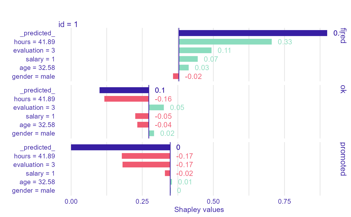
  pl1 <- plot(ive_rf, bar_width = 4)
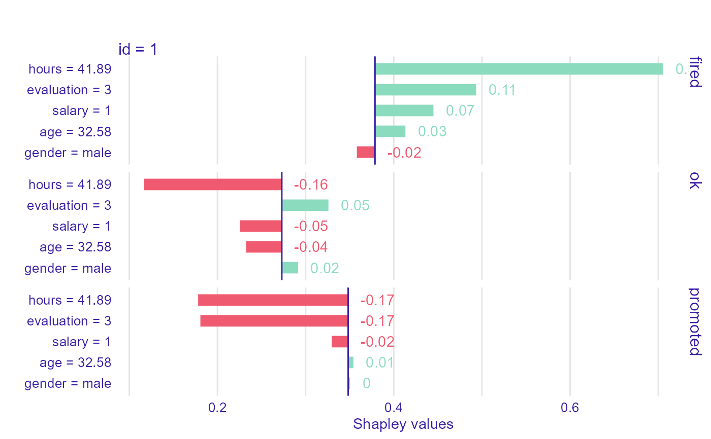
  pl2 <- plot(ive_rf, bar_width = 4, show_predicted = FALSE)
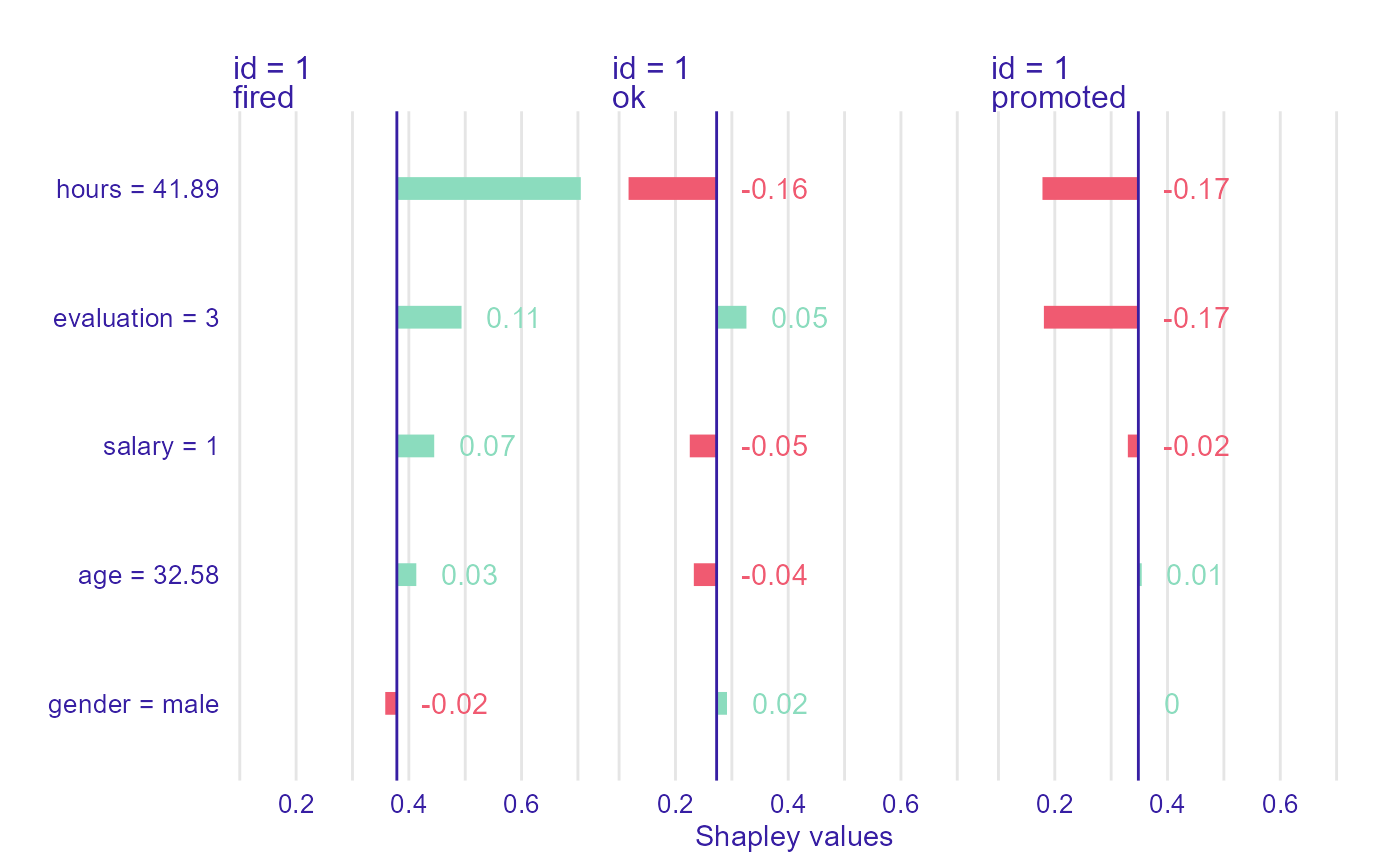
  pl3 <- plot(ive_rf, bar_width = 4, show_predicted = FALSE,
              cols = c("id","ylevel"), rows = "label")
  print(pl1)
  print(pl2)
  print(pl3)
} else {
    print('Python testing environment is required.')
}