Introduction

The shapper is an R package which ports the shap python library in R. For details and examples see shapper repository on github and shapper website.

SHAP (SHapley Additive exPlanations) is a method to explain predictions of any machine learning model. For more details about this method see shap repository on github.

Install shaper and shap

R package shapper

library("shapper")

Python library shap

To run shapper python library shap is required. It can be installed both by python or R. To install it throught R, you an use function install_shap from the shapper package.

shapper::install_shap()

Load data sets

The example usage is presented on the titanic dataset form the R package DALEX.

library("DALEX")
titanic_train <- titanic[,c("survived", "class", "gender", "age", "sibsp", "parch", "fare", "embarked")]
titanic_train$survived <- factor(titanic_train$survived)
titanic_train$gender <- factor(titanic_train$gender)
titanic_train$embarked <- factor(titanic_train$embarked)
titanic_train <- na.omit(titanic_train)
head(titanic_train)

##   survived class gender age sibsp parch  fare    embarked
## 1       no   3rd   male  42     0     0  7.11 Southampton
## 2       no   3rd   male  13     0     2 20.05 Southampton
## 3       no   3rd   male  16     1     1 20.05 Southampton
## 4      yes   3rd female  39     1     1 20.05 Southampton
## 5      yes   3rd female  16     0     0  7.13 Southampton
## 6      yes   3rd   male  25     0     0  7.13 Southampton

Let’s build a model

library("randomForest")
set.seed(123)
model_rf <- randomForest(survived ~ . , data = titanic_train)
model_rf

## 
## Call:
##  randomForest(formula = survived ~ ., data = titanic_train) 
##                Type of random forest: classification
##                      Number of trees: 500
## No. of variables tried at each split: 2
## 
##         OOB estimate of  error rate: 18.59%
## Confusion matrix:
##       no yes class.error
## no  1374  96  0.06530612
## yes  309 400  0.43582511

Prediction to be explained

Let’s assume that we want to explain the prediction of a particular observation (male, 8 years old, traveling 1-st class embarked at C, without parents and siblings.

new_passanger <- data.frame(
            class = factor("1st", levels = c("1st", "2nd", "3rd", "deck crew", "engineering crew", "restaurant staff", "victualling crew")),
            gender = factor("male", levels = c("female", "male")),
            age = 8,
            sibsp = 0,
            parch = 0,
            fare = 72,
            embarked = factor("Cherbourg", levels = c("Belfast", "Cherbourg", "Queenstown", "Southampton"))
)

Here shapper starts

To use the function shap() function (alias for individual_variable_effect()) we need four elements

a model,
a data set,
a function that calculated scores (predict function),
an instance (or instances) to be explained.

The shap() function can be used directly with these four arguments, but for the simplicity here we are using the DALEX package with preimplemented predict functions.

library("DALEX")
exp_rf <- explain(model_rf, data = titanic_train[,-1], y = as.numeric(titanic_train[,1])-1)

## Preparation of a new explainer is initiated
##   -> model label       :  randomForest  ( [33m default [39m )
##   -> data              :  2179  rows  7  cols 
##   -> target variable   :  2179  values 
##   -> predict function  :  yhat.randomForest  will be used ( [33m default [39m )
##   -> predicted values  :  No value for predict function target column. ( [33m default [39m )
##   -> model_info        :  package randomForest , ver. 4.6.14 , task classification ( [33m default [39m ) 
##   -> predicted values  :  numerical, min =  0 , mean =  0.2411381 , max =  1  
##   -> residual function :  difference between y and yhat ( [33m default [39m )
##   -> residuals         :  numerical, min =  -0.906 , mean =  0.08424048 , max =  1  
##  [32m A new explainer has been created! [39m

The explainer is an object that wraps up a model and meta-data. Meta data consists of, at least, the data set used to fit model and observations to explain.

And now it’s enough to generate SHAP attributions with explainer for RF model.

library("shapper")
ive_rf <- shap(exp_rf, new_observation = new_passanger)
ive_rf

##     class gender age sibsp parch fare  embarked _id_ _ylevel_ _yhat_
## 1     1st   male   8     0     0   72 Cherbourg    1           0.516
## 1.1   1st   male   8     0     0   72 Cherbourg    1           0.516
## 1.2   1st   male   8     0     0   72 Cherbourg    1           0.516
## 1.3   1st   male   8     0     0   72 Cherbourg    1           0.516
## 1.4   1st   male   8     0     0   72 Cherbourg    1           0.516
## 1.5   1st   male   8     0     0   72 Cherbourg    1           0.516
##     _yhat_mean_ _vname_ _attribution_ _sign_      _label_
## 1     0.2411381   class   0.100631854      + randomForest
## 1.1   0.2411381  gender  -0.103475978      - randomForest
## 1.2   0.2411381     age   0.208512839      + randomForest
## 1.3   0.2411381   sibsp   0.004010866      + randomForest
## 1.4   0.2411381   parch  -0.018113978      - randomForest
## 1.5   0.2411381    fare   0.024801427      + randomForest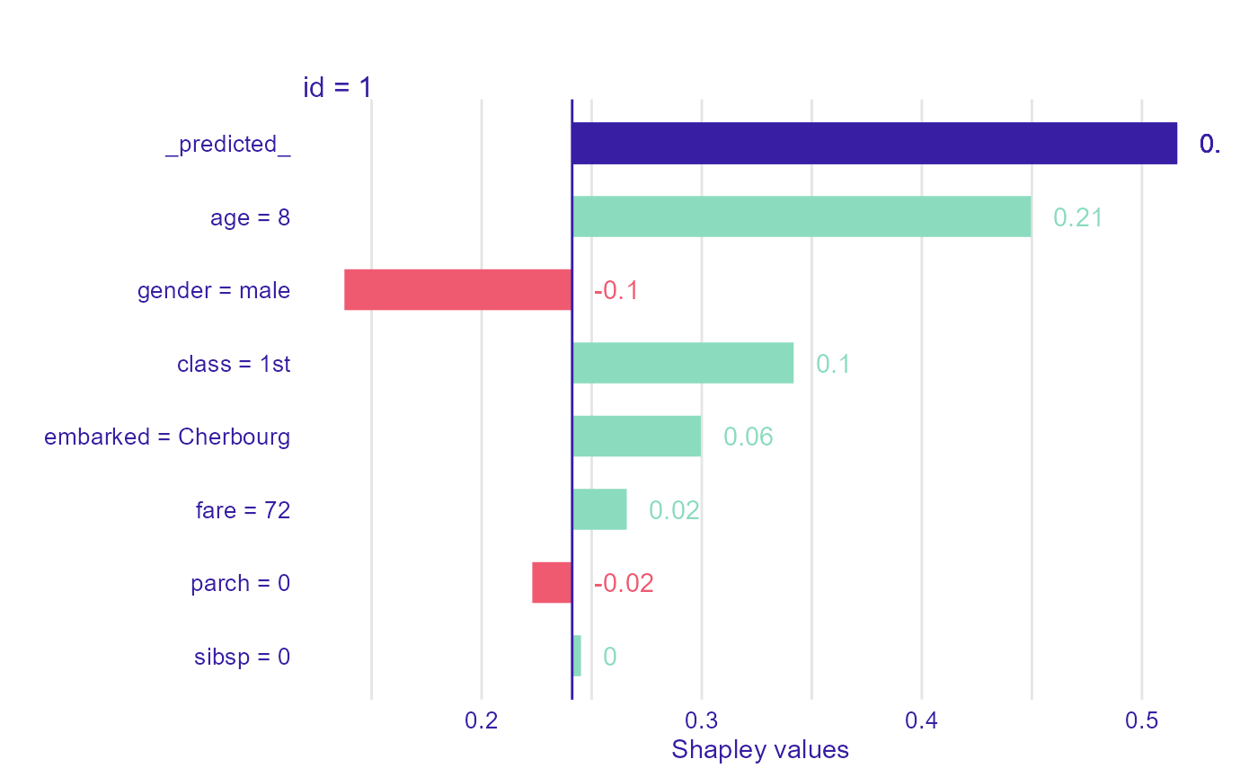

Plotting results

plot(ive_rf)

How to use shapper for regression

Alicja Gosiewska

2021-07-01