Disaggregated partial dependencies, see reference. The plot method supports
up to two grouping variables via BY.
ice(object, ...)

# Default S3 method
ice(
  object,
  v,
  X,
  pred_fun = stats::predict,
  BY = NULL,
  grid = NULL,
  grid_size = 49L,
  trim = c(0.01, 0.99),
  strategy = c("uniform", "quantile"),
  na.rm = TRUE,
  n_max = 100L,
  ...
)

# S3 method for class 'ranger'
ice(
  object,
  v,
  X,
  pred_fun = NULL,
  BY = NULL,
  grid = NULL,
  grid_size = 49L,
  trim = c(0.01, 0.99),
  strategy = c("uniform", "quantile"),
  na.rm = TRUE,
  n_max = 100L,
  survival = c("chf", "prob"),
  ...
)

# S3 method for class 'explainer'
ice(
  object,
  v = v,
  X = object[["data"]],
  pred_fun = object[["predict_function"]],
  BY = NULL,
  grid = NULL,
  grid_size = 49L,
  trim = c(0.01, 0.99),
  strategy = c("uniform", "quantile"),
  na.rm = TRUE,
  n_max = 100L,
  ...
)
Arguments
- object
Fitted model object.
- ...
Additional arguments passed to
pred_fun(object, X, ...), for instancetype = "response"in aglm()model, orreshape = TRUEin a multiclass XGBoost model.- v
One or more column names over which you want to calculate the ICE.
- X
A data.frame or matrix serving as background dataset.
- pred_fun
Prediction function of the form
function(object, X, ...), providing \(K \ge 1\) predictions per row. Its first argument represents the modelobject, its second argument a data structure likeX. Additional arguments (such astype = "response"in a GLM, orreshape = TRUEin a multiclass XGBoost model) can be passed via.... The default,stats::predict(), will work in most cases.- BY
Optional grouping vector/matrix/data.frame (up to two columns), or up to two column names. Unlike with
partial_dep(), these variables are not binned. The first variable is visualized on the color scale, while the second one goes into afacet_wrap(). Thus, make sure that the second variable is discrete.- grid
Evaluation grid. A vector (if
length(v) == 1L), or a matrix/data.frame otherwise. IfNULL, calculated viamultivariate_grid().- grid_size
Controls the approximate grid size. If
xhas p columns, then each (non-discrete) column will be reduced to about the p-th root ofgrid_sizevalues.- trim
The default
c(0.01, 0.99)means that values outside the 1% and 99% quantiles of non-discrete numeric columns are removed before calculation of grid values. Set to0:1for no trimming.- strategy
How to find grid values of non-discrete numeric columns? Either "uniform" or "quantile", see description of
univariate_grid().- na.rm
Should missing values be dropped from the grid? Default is
TRUE.- n_max
If
Xhas more thann_maxrows, a random sample ofn_maxrows is selected fromX. In this case, set a random seed for reproducibility.- survival
Should cumulative hazards ("chf", default) or survival probabilities ("prob") per time be predicted? Only in
ranger()survival models.
Value
An object of class "ice" containing these elements:
data: data.frame containing the ice values.grid: Vector, matrix or data.frame of grid values.v: Same as inputv.K: Number of columns of prediction matrix.pred_names: Column names of prediction matrix.by_names: Column name(s) of grouping variable(s) (orNULL).
Methods (by class)
ice(default): Default method.ice(ranger): Method for "ranger" models.ice(explainer): Method for DALEX "explainer".
References
Goldstein, Alex, and Adam Kapelner and Justin Bleich and Emil Pitkin. Peeking inside the black box: Visualizing statistical learning with plots of individual conditional expectation. Journal of Computational and Graphical Statistics, 24, no. 1 (2015): 44-65.
Examples
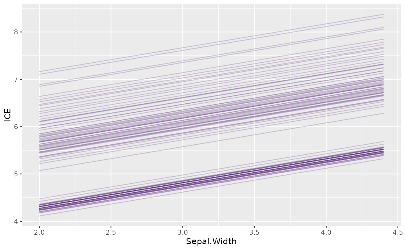
# MODEL 1: Linear regression
fit <- lm(Sepal.Length ~ . + Species * Petal.Length, data = iris)
plot(ice(fit, v = "Sepal.Width", X = iris))
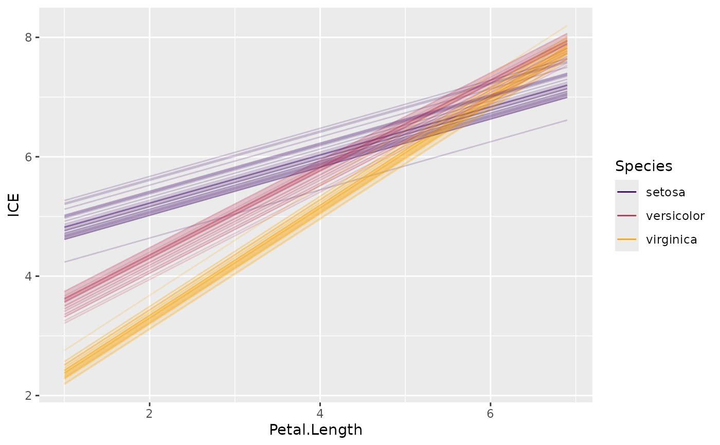
 # Stratified by one variable
ic <- ice(fit, v = "Petal.Length", X = iris, BY = "Species")
ic
#> 'ice' object (4300 rows). Extract via $data. Top rows:
#>
#> obs_ Petal.Length y Species
#> 1 1 1 4.644850 setosa
#> 2 2 1 4.616713 setosa
#> 3 3 1 4.717621 setosa
plot(ic)
# Stratified by one variable
ic <- ice(fit, v = "Petal.Length", X = iris, BY = "Species")
ic
#> 'ice' object (4300 rows). Extract via $data. Top rows:
#>
#> obs_ Petal.Length y Species
#> 1 1 1 4.644850 setosa
#> 2 2 1 4.616713 setosa
#> 3 3 1 4.717621 setosa
plot(ic)
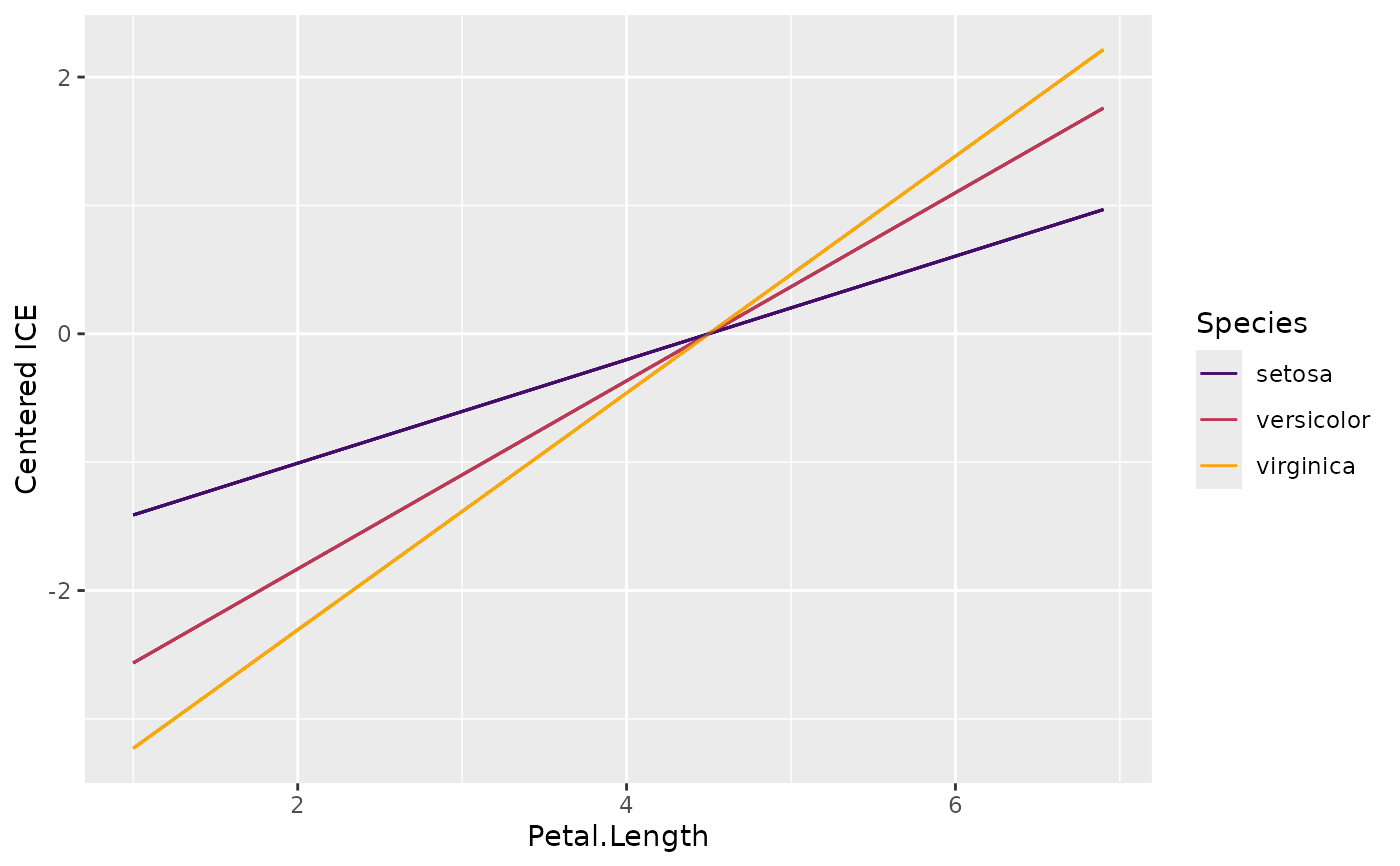
 plot(ic, center = TRUE)
 if (FALSE) { # \dontrun{
# Stratified by two variables (the second one goes into facets)
ic <- ice(fit, v = "Petal.Length", X = iris, BY = c("Petal.Width", "Species"))
plot(ic)
plot(ic, center = TRUE)
# MODEL 2: Multi-response linear regression
fit <- lm(as.matrix(iris[, 1:2]) ~ Petal.Length + Petal.Width * Species, data = iris)
ic <- ice(fit, v = "Petal.Width", X = iris, BY = iris$Species)
plot(ic)
plot(ic, center = TRUE)
plot(ic, swap_dim = TRUE)
} # }
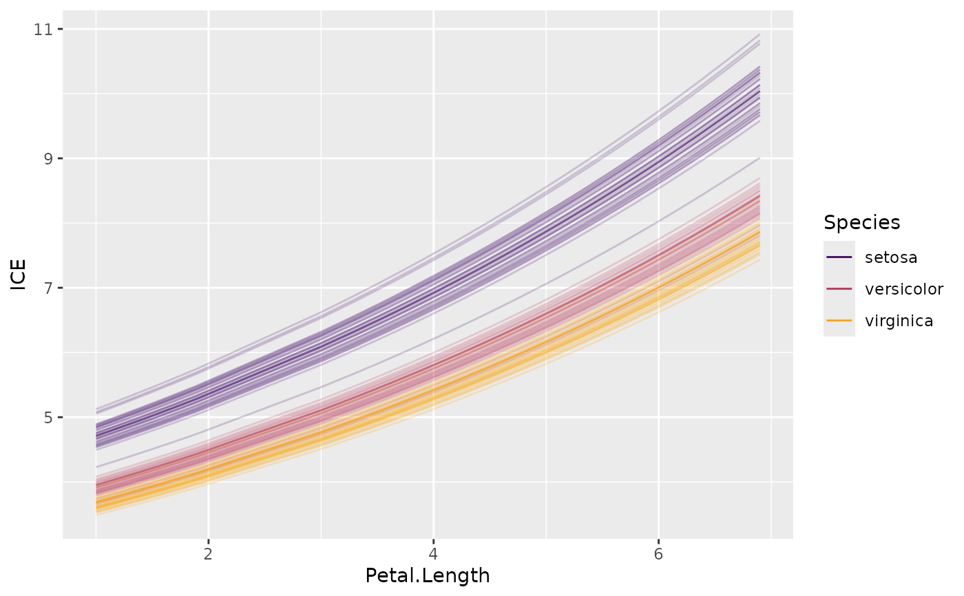
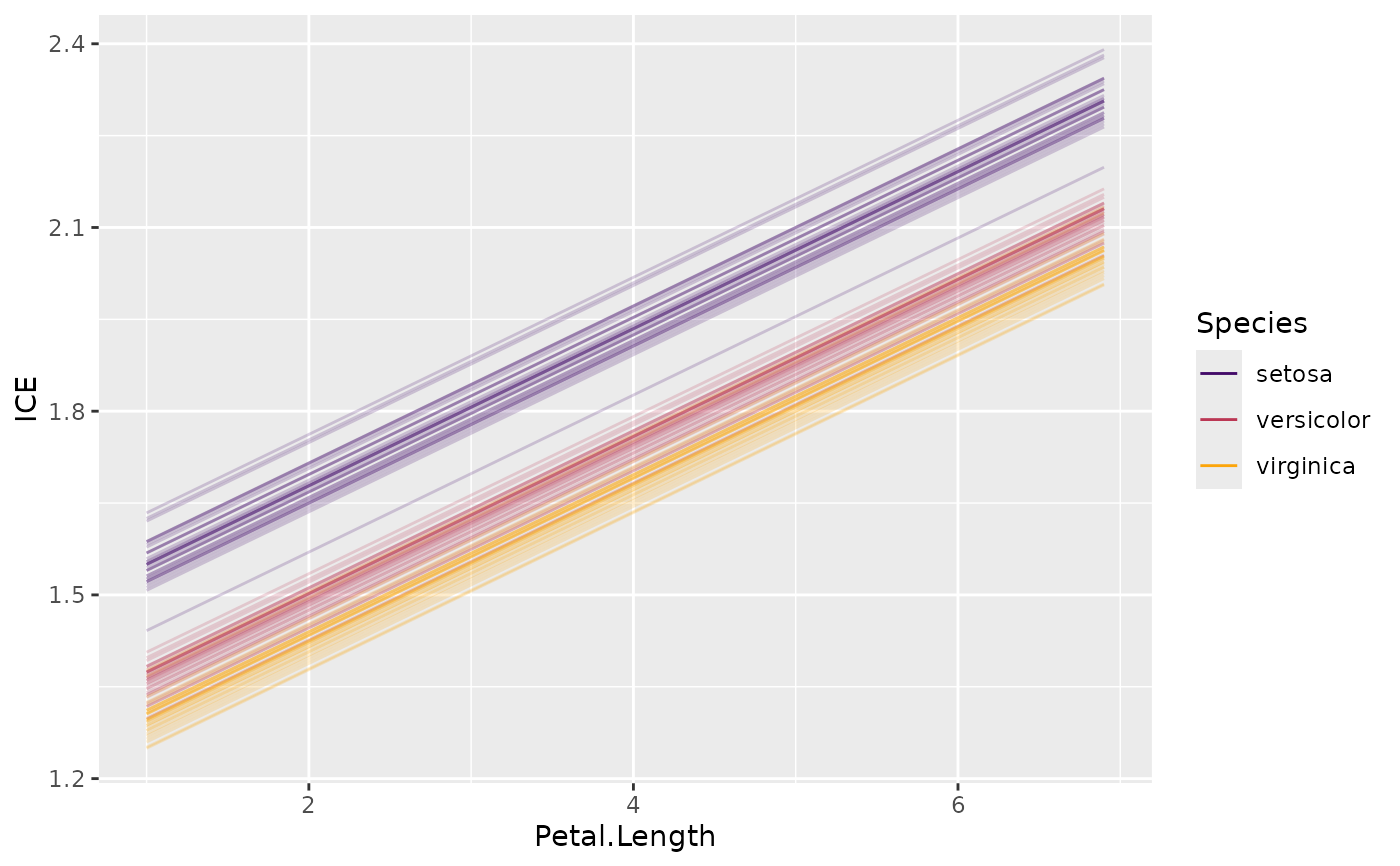
# MODEL 3: Gamma GLM -> pass options to predict() via ...
fit <- glm(Sepal.Length ~ ., data = iris, family = Gamma(link = log))
plot(ice(fit, v = "Petal.Length", X = iris, BY = "Species"))
if (FALSE) { # \dontrun{
# Stratified by two variables (the second one goes into facets)
ic <- ice(fit, v = "Petal.Length", X = iris, BY = c("Petal.Width", "Species"))
plot(ic)
plot(ic, center = TRUE)
# MODEL 2: Multi-response linear regression
fit <- lm(as.matrix(iris[, 1:2]) ~ Petal.Length + Petal.Width * Species, data = iris)
ic <- ice(fit, v = "Petal.Width", X = iris, BY = iris$Species)
plot(ic)
plot(ic, center = TRUE)
plot(ic, swap_dim = TRUE)
} # }
# MODEL 3: Gamma GLM -> pass options to predict() via ...
fit <- glm(Sepal.Length ~ ., data = iris, family = Gamma(link = log))
plot(ice(fit, v = "Petal.Length", X = iris, BY = "Species"))
 plot(ice(fit, v = "Petal.Length", X = iris, type = "response", BY = "Species"))