Average Loss — average

Calculates the average loss of a model on a given dataset, optionally grouped by a variable. Use plot() to visualize the results.

average_loss(object, ...)

# Default S3 method
average_loss(
  object,
  X,
  y,
  pred_fun = stats::predict,
  loss = "squared_error",
  agg_cols = FALSE,
  BY = NULL,
  by_size = 4L,
  w = NULL,
  ...
)

# S3 method for class 'ranger'
average_loss(
  object,
  X,
  y,
  pred_fun = function(m, X, ...) stats::predict(m, X, ...)$predictions,
  loss = "squared_error",
  agg_cols = FALSE,
  BY = NULL,
  by_size = 4L,
  w = NULL,
  ...
)

# S3 method for class 'explainer'
average_loss(
  object,
  X = object[["data"]],
  y = object[["y"]],
  pred_fun = object[["predict_function"]],
  loss = "squared_error",
  agg_cols = FALSE,
  BY = NULL,
  by_size = 4L,
  w = object[["weights"]],
  ...
)

Arguments

object: Fitted model object.
...: Additional arguments passed to pred_fun(object, X, ...), for instance type = "response" in a glm() model, or reshape = TRUE in a multiclass XGBoost model.
X: A data.frame or matrix serving as background dataset.
y: Vector/matrix of the response, or the corresponding column names in X.
pred_fun: Prediction function of the form function(object, X, ...), providing \(K \ge 1\) predictions per row. Its first argument represents the model object, its second argument a data structure like X. Additional arguments (such as type = "response" in a GLM, or reshape = TRUE in a multiclass XGBoost model) can be passed via .... The default, stats::predict(), will work in most cases.
loss: One of "squared_error", "logloss", "mlogloss", "poisson", "gamma", or "absolute_error". Alternatively, a loss function can be provided that turns observed and predicted values into a numeric vector or matrix of unit losses of the same length as X. For "mlogloss", the response y can either be a dummy matrix or a discrete vector. The latter case is handled via a fast version of model.matrix(~ as.factor(y) + 0). For "squared_error", the response can be a factor with levels in column order of the predictions. In this case, squared error is evaluated for each one-hot-encoded column.
agg_cols: Should multivariate losses be summed up? Default is FALSE. In combination with the squared error loss, agg_cols = TRUE gives the Brier score for (probabilistic) classification.
BY: Optional grouping vector or column name. Numeric BY variables with more than by_size disjoint values will be binned into by_size quantile groups of similar size.
by_size: Numeric BY variables with more than by_size unique values will be binned into quantile groups. Only relevant if BY is not NULL.
w: Optional vector of case weights. Can also be a column name of X.

Value

An object of class "hstats_matrix" containing these elements:

M: Matrix of statistics (one column per prediction dimension), or NULL.
SE: Matrix with standard errors of M, or NULL. Multiply with sqrt(m_rep) to get standard deviations instead. Currently, supported only for perm_importance().
m_rep: The number of repetitions behind standard errors SE, or NULL. Currently, supported only for perm_importance().
statistic: Name of the function that generated the statistic.
description: Description of the statistic.

Methods (by class)

average_loss(default): Default method.
average_loss(ranger): Method for "ranger" models.
average_loss(explainer): Method for DALEX "explainer".

Losses

The default loss is the "squared_error". Other choices:

"absolute_error": The absolute error is the loss corresponding to median regression.
"poisson": Unit Poisson deviance, i.e., the loss function used in Poisson regression. Actual values y and predictions must be non-negative.
"gamma": Unit gamma deviance, i.e., the loss function of Gamma regression. Actual values y and predictions must be positive.
"logloss": The Log Loss is the loss function used in logistic regression, and the top choice in probabilistic binary classification. Responses y and predictions must be between 0 and 1. Predictions represent probabilities of having a "1".
"mlogloss": Multi-Log-Loss is the natural loss function in probabilistic multi-class situations. If there are K classes and n observations, the predictions form a (n x K) matrix of probabilities (with row-sums 1). The observed values y are either passed as (n x K) dummy matrix, or as discrete vector with corresponding levels. The latter case is turned into a dummy matrix by a fast version of model.matrix(~ as.factor(y) + 0).
A function with signature f(actual, predicted), returning a numeric vector or matrix of the same length as the input.

Examples

# MODEL 1: Linear regression
fit <- lm(Sepal.Length ~ ., data = iris)
average_loss(fit, X = iris, y = "Sepal.Length")
#> Average loss
#> [1] 0.09037657
average_loss(fit, X = iris, y = iris$Sepal.Length, BY = iris$Sepal.Width)
#> Average loss
#>    [2,2.8]    (2.8,3]    (3,3.3]  (3.3,4.4] 
#> 0.08934441 0.09847409 0.09612552 0.07914772 
average_loss(fit, X = iris, y = "Sepal.Length", BY = "Sepal.Width")
#> Average loss
#>    [2,2.8]    (2.8,3]    (3,3.3]  (3.3,4.4] 
#> 0.08934441 0.09847409 0.09612552 0.07914772 

# MODEL 2: Multi-response linear regression
fit <- lm(as.matrix(iris[, 1:2]) ~ Petal.Length + Petal.Width + Species, data = iris)
average_loss(fit, X = iris, y = iris[, 1:2])
#> Average loss
#> Sepal.Length  Sepal.Width 
#>   0.11120993   0.08472089 
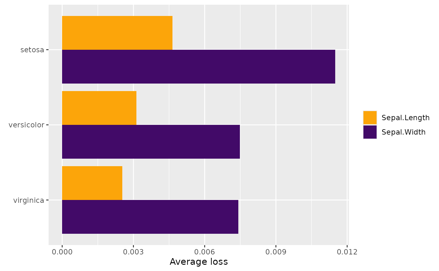
L <- average_loss(
  fit, X = iris, y = iris[, 1:2], loss = "gamma", BY = "Species"
)
L
#> Average loss
#>            Sepal.Length Sepal.Width
#> setosa      0.004646018 0.011500586
#> versicolor  0.003121888 0.007489254
#> virginica   0.002525590 0.007419552
plot(L)