Print Model Drift Data Frame

Print Model Drift Data Frame

# S3 method for model_drift
print(x, max_length = 25, ...)

Arguments

x	an object of the class `model_drift`
max_length	length of the first column, by default 25
...	other arguments, currently ignored

Value

this function prints a data frame with a nicer format

Examples

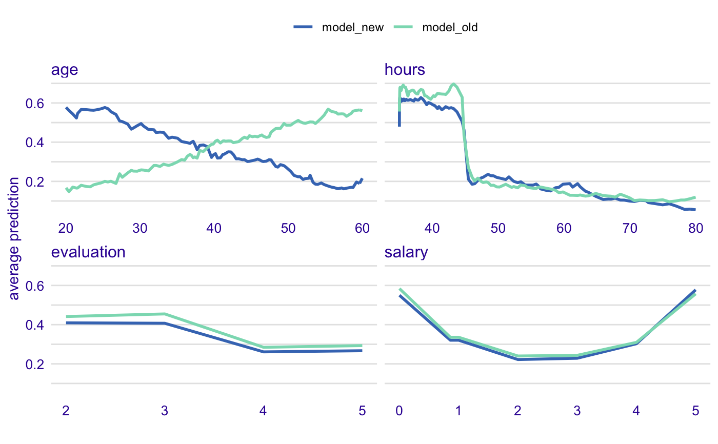
 library("DALEX")
 model_old <- lm(m2.price ~ ., data = apartments)
 model_new <- lm(m2.price ~ ., data = apartments_test[1:1000,])
 calculate_model_drift(model_old, model_new,
                  apartments_test[1:1000,],
                  apartments_test[1:1000,]$m2.price)
#>                   Variable    Shift  Scaled
#>   -----------------------------------------------
#>                      floor   170.48    19.1  .
#>                   no.rooms   168.87    18.9  .
#>                    surface   162.15    18.2  .
#>                   m2.price   169.04    18.9  .
#>          construction.year   168.95    18.9  .
 
 library("ranger")
 predict_function <- function(m,x,...) predict(m, x, ...)$predictions
 model_old <- ranger(m2.price ~ ., data = apartments)
 model_new <- ranger(m2.price ~ ., data = apartments_test)
 calculate_model_drift(model_old, model_new,
                  apartments_test,
                  apartments_test$m2.price,
                  predict_function = predict_function)
#>                   Variable    Shift  Scaled
#>   -----------------------------------------------
#>                      floor   112.89    12.5  .
#>                   no.rooms    61.11     6.8  
#>                    surface    41.19     4.6  
#>                   m2.price    72.49     8.1  
#>          construction.year    84.20     9.4  

 # here we compare model created on male data
 # with model applied to female data
 # there is interaction with age, and it is detected here
 predict_function <- function(m,x,...) predict(m, x, ..., probability=TRUE)$predictions[,1]
 data_old = HR[HR$gender == "male", -1]
 data_new = HR[HR$gender == "female", -1]
 model_old <- ranger(status ~ ., data = data_old, probability=TRUE)
 model_new <- ranger(status ~ ., data = data_new, probability=TRUE)
 calculate_model_drift(model_old, model_new,
                  HR_test,
                  HR_test$status == "fired",
                  predict_function = predict_function)
#>                   Variable    Shift  Scaled
#>   -----------------------------------------------
#>                     salary     0.11    22.2  *
#>                 evaluation     0.06    13.2  .
#>                        age     0.30    62.2  ***
#>                      hours     0.05    10.4  .

 # plot it
 library("ingredients")
 prof_old <- partial_dependency(model_old,
                                     data = data_new[1:1000,],
                                     label = "model_old",
                                     predict_function = predict_function,
                                     grid_points = 101,
                                     variable_splits = NULL)
 prof_new <- partial_dependency(model_new,
                                     data = data_new[1:1000,],
                                     label = "model_new",
                                     predict_function = predict_function,
                                     grid_points = 101,
                                     variable_splits = NULL)
 plot(prof_old, prof_new, color = "_label_")