Plots Individual Variable Profile Explanations
Function 'plot.individual_variable_profile_explainer' plots Individual Variable Profiles for selected observations. Various parameters help to decide what should be plotted, profiles, aggregated profiles, points or rugs.
# S3 method for individual_variable_profile_explainer
plot(x, ..., size = 1,
  alpha = 0.3, color = "black", size_points = 2, alpha_points = 1,
  color_points = color, size_rugs = 0.5, alpha_rugs = 1,
  color_rugs = color, size_residuals = 1, alpha_residuals = 1,
  color_residuals = color, only_numerical = TRUE,
  show_profiles = TRUE, show_observations = TRUE, show_rugs = FALSE,
  show_residuals = FALSE, aggregate_profiles = NULL,
  facet_ncol = NULL, selected_variables = NULL)
Arguments
| x | a ceteris paribus explainer produced with function `individual_variable_profile()` |
|---|---|
| ... | other explainers that shall be plotted together |
| size | a numeric. Size of lines to be plotted |
| alpha | a numeric between 0 and 1. Opacity of lines |
| color | a character. Either name of a color or name of a variable that should be used for coloring |
| size_points | a numeric. Size of points to be plotted |
| alpha_points | a numeric between 0 and 1. Opacity of points |
| color_points | a character. Either name of a color or name of a variable that should be used for coloring |
| size_rugs | a numeric. Size of rugs to be plotted |
| alpha_rugs | a numeric between 0 and 1. Opacity of rugs |
| color_rugs | a character. Either name of a color or name of a theme_mi2variable that should be used for coloring |
| size_residuals | a numeric. Size of line and points to be plotted for residuals |
| alpha_residuals | a numeric between 0 and 1. Opacity of points and lines for residuals |
| color_residuals | a character. Either name of a color or name of a variable that should be used for coloring for residuals |
| only_numerical | a logical. If TRUE then only numerical variables will be plotted. If FALSE then only categorical variables will be plotted. |
| show_profiles | a logical. If TRUE then profiles will be plotted. Either individual or aggregate (see `aggregate_profiles`) |
| show_observations | a logical. If TRUE then individual observations will be marked as points |
| show_rugs | a logical. If TRUE then individual observations will be marked as rugs |
| show_residuals | a logical. If TRUE then residuals will be plotted as a line ended with a point |
| aggregate_profiles | function. If NULL (default) then individual profiles will be plotted. If a function (e.g. mean or median) then profiles will be aggregated and only the aggregate profile will be plotted |
| facet_ncol | number of columns for the `facet_wrap()` |
| selected_variables | if not NULL then only `selected_variables` will be presented |
Value
a ggplot2 object
Examples
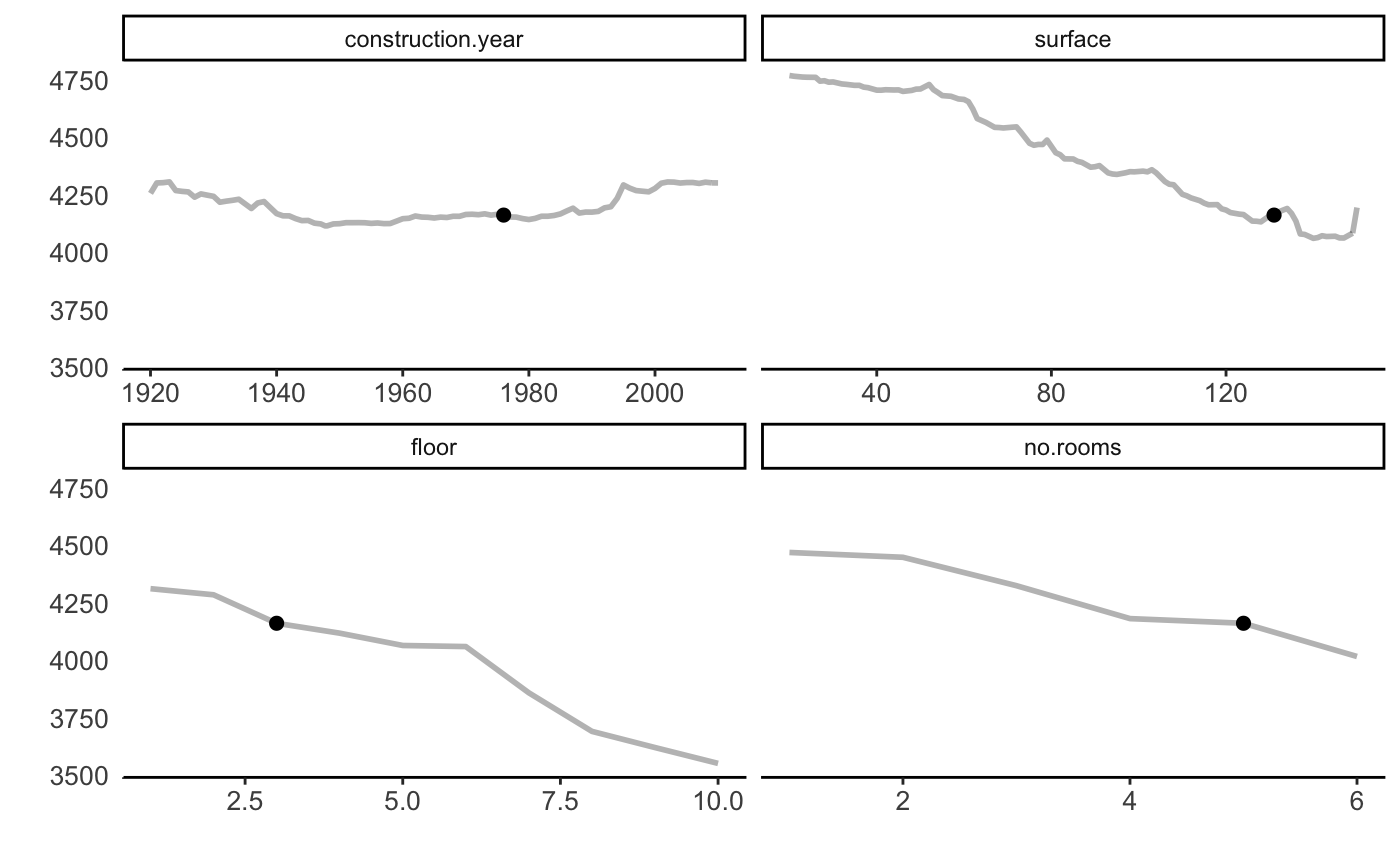
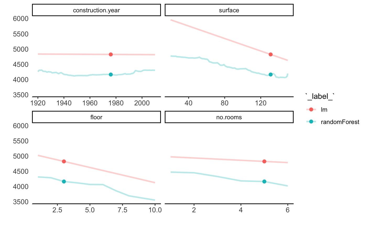
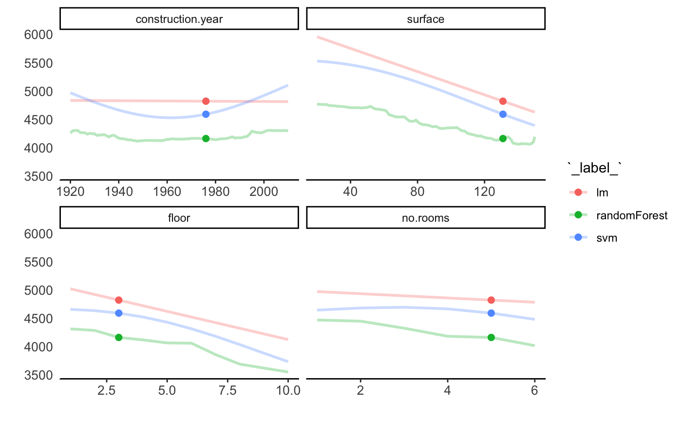
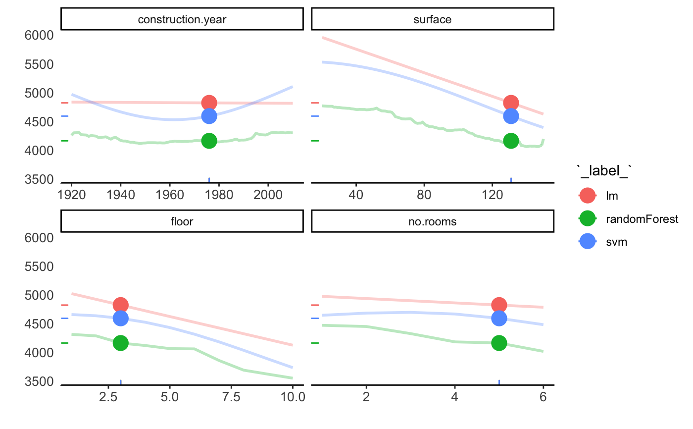
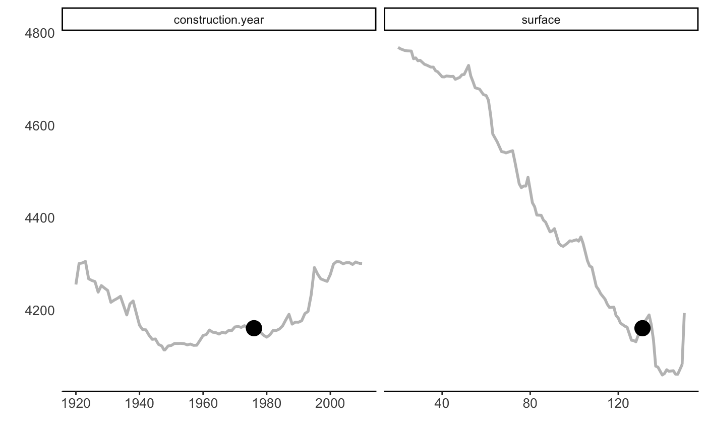
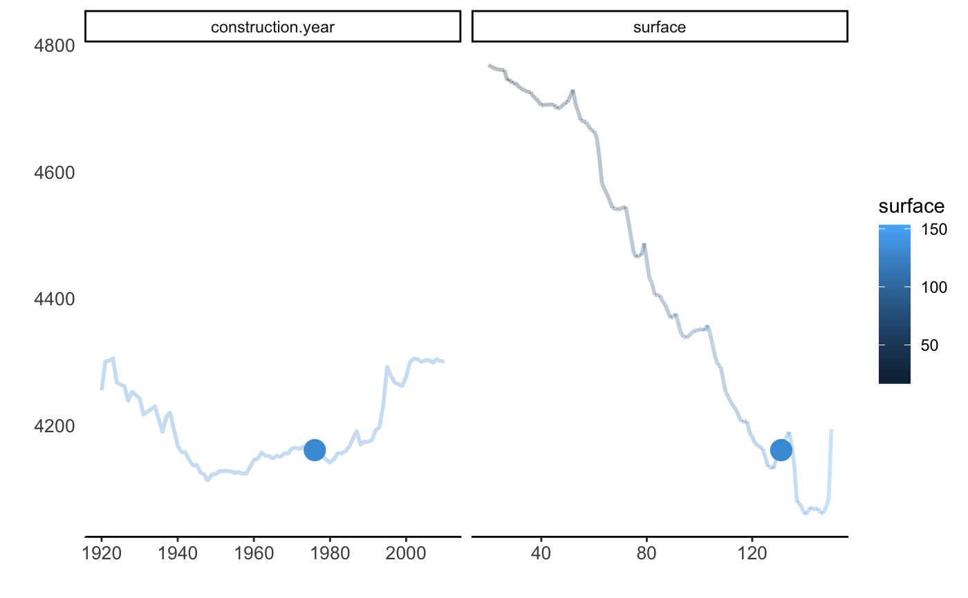
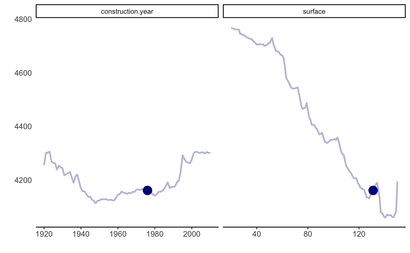
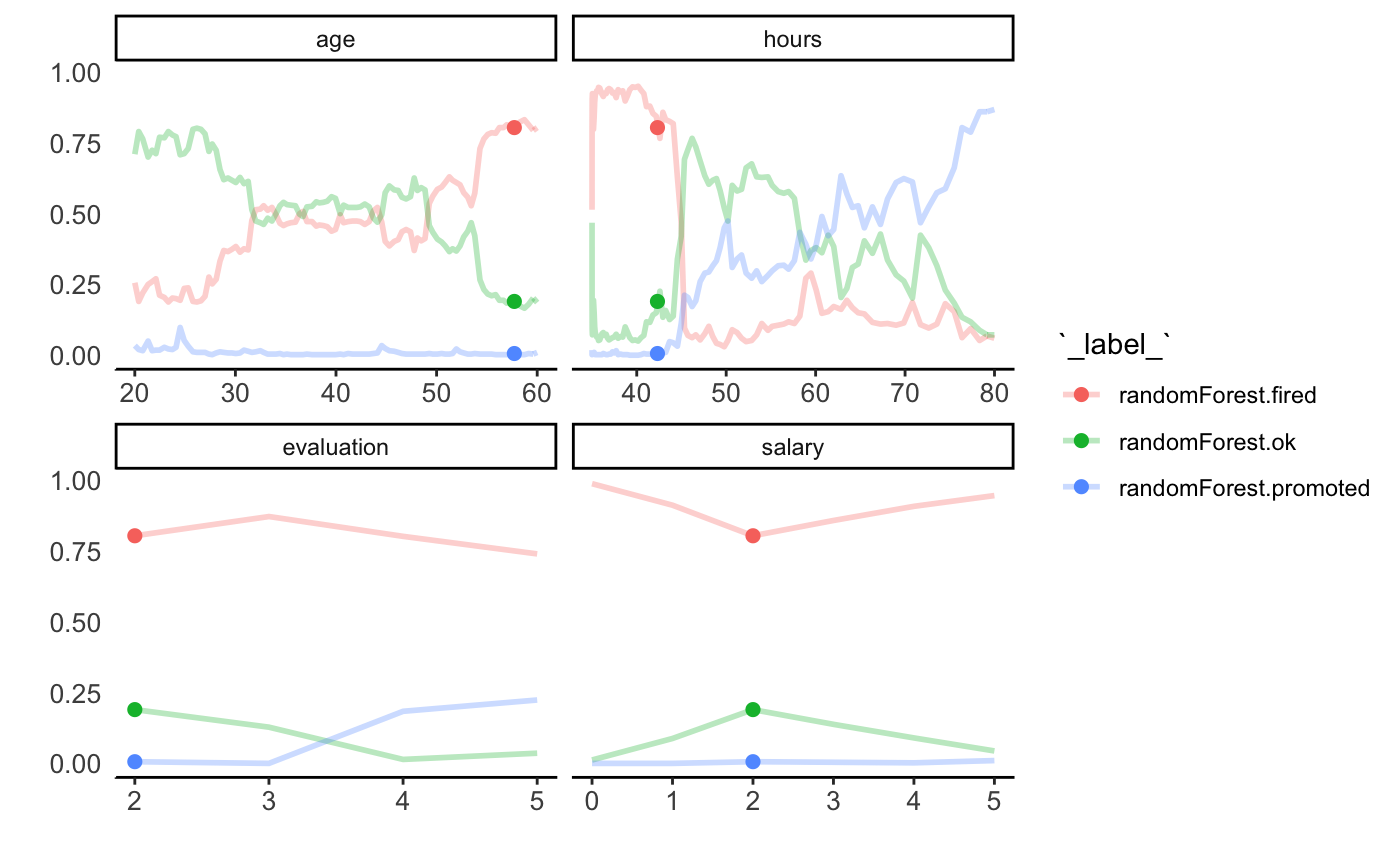
library("DALEX2")library("randomForest") set.seed(59) apartments_rf <- randomForest(m2.price ~ construction.year + surface + floor + no.rooms + district, data = apartments) explainer_rf <- explain(apartments_rf, data = apartments_test[,2:6], y = apartments_test$m2.price) apartments_lm <- lm(m2.price ~ construction.year + surface + floor + no.rooms + district, data = apartments) explainer_lm <- explain(apartments_lm, data = apartments_test[,2:6], y = apartments_test$m2.price) library("e1071") apartments_svm <- svm(m2.price ~ construction.year + surface + floor + no.rooms + district, data = apartments) explainer_svm <- explain(apartments_svm, data = apartments_test[,2:6], y = apartments_test$m2.price) # individual explanations my_apartment <- apartments_test[1, ] # for random forest lp_rf <- individual_variable_profile(explainer_rf, my_apartment) lp_rf#> Top profiles : #> construction.year surface floor no.rooms district _yhat_ #> 1001 1920 131 3 5 Srodmiescie 4255.354 #> 1001.1 1921 131 3 5 Srodmiescie 4300.702 #> 1001.2 1922 131 3 5 Srodmiescie 4301.926 #> 1001.3 1923 131 3 5 Srodmiescie 4305.352 #> 1001.4 1923 131 3 5 Srodmiescie 4305.352 #> 1001.5 1924 131 3 5 Srodmiescie 4267.723 #> _vname_ _ids_ _label_ #> 1001 construction.year 1001 randomForest #> 1001.1 construction.year 1001 randomForest #> 1001.2 construction.year 1001 randomForest #> 1001.3 construction.year 1001 randomForest #> 1001.4 construction.year 1001 randomForest #> 1001.5 construction.year 1001 randomForest #> #> #> Top observations: #> construction.year surface floor no.rooms district _yhat_ _label_ #> 1001 1976 131 3 5 Srodmiescie 4160.84 randomForest #> _ids_ #> 1001 1plot(lp_rf)# for others lp_lm <- individual_variable_profile(explainer_lm, my_apartment) plot(lp_rf, lp_lm, color = "_label_")# for others lp_svm <- individual_variable_profile(explainer_svm, my_apartment) plot(lp_rf, lp_lm, lp_svm, color = "_label_")# more parameters plot(lp_rf, lp_lm, lp_svm, color = "_label_", show_profiles = TRUE, show_observations = TRUE, show_rugs = TRUE, alpha = 0.3, alpha_points = 1, size_points = 5, size_rugs = 0.5)plot(lp_rf, show_profiles = TRUE, show_observations = TRUE, color = "black", selected_variables = c("construction.year", "surface"), alpha = 0.3, alpha_points = 1, alpha_residuals = 0.5, size_points = 5, size_rugs = 0.5)plot(lp_rf, show_profiles = TRUE, show_observations = TRUE, color = "surface", selected_variables = c("construction.year", "surface"), alpha = 0.3, alpha_points = 1, alpha_residuals = 0.5, size_points = 5, size_rugs = 0.5)plot(lp_rf, show_profiles = TRUE, show_observations = TRUE, color = "darkblue", aggregate_profiles = mean, selected_variables = c("construction.year", "surface"), alpha = 0.3, alpha_points = 1, alpha_residuals = 0.5, size_points = 5, size_rugs = 0.5)# -------- # multiclass HR_rf <- randomForest(status ~ . , data = HR) explainer_rf <- explain(HR_rf, data = HRTest, y = HRTest) my_HR <- HRTest[1, ] lp_rf <- individual_variable_profile(explainer_rf, my_HR) lp_rf#> Top profiles : #> gender age hours evaluation salary status _vname_ _ids_ _yhat_ #> 1 male 57.72683 42.31527 2 2 fired gender 1 0.804 #> 1.1 female 57.72683 42.31527 2 2 fired gender 1 0.226 #> 11 male 20.00212 42.31527 2 2 fired age 1 0.256 #> 1.110 male 20.39166 42.31527 2 2 fired age 1 0.190 #> 1.2 male 20.78820 42.31527 2 2 fired age 1 0.220 #> 1.3 male 21.32338 42.31527 2 2 fired age 1 0.250 #> _label_ #> 1 randomForest.fired #> 1.1 randomForest.fired #> 11 randomForest.fired #> 1.110 randomForest.fired #> 1.2 randomForest.fired #> 1.3 randomForest.fired #> #> #> Top observations: #> gender age hours evaluation salary status _yhat_ #> 1 male 57.72683 42.31527 2 2 fired 0.804 #> 1.1 male 57.72683 42.31527 2 2 fired 0.190 #> 1.2 male 57.72683 42.31527 2 2 fired 0.006 #> _label_ _ids_ #> 1 randomForest.fired 1 #> 1.1 randomForest.ok 1 #> 1.2 randomForest.promoted 1plot(lp_rf, color = "_label_")