Half-Normal plot

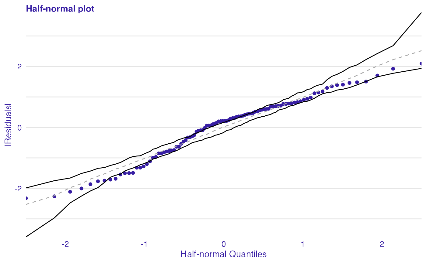
The half-normal plot is one of the tools designed to evaluate the goodness of fit of a statistical models. It is a graphical method for comparing two probability distributions by plotting their quantiles against each other. Points on the plot correspond to ordered absolute values of model diagnostic (i.e. standardized residuals) plotted against theoretical order statistics from a half-normal distribution.

plot_halfnormal(object, ..., quantiles = FALSE, sim = 99)

plotHalfNormal(object, ..., quantiles = FALSE, sim = 99)

Arguments

object	An object of class auditor_model_halfnormal created with model_halfnormal function.
...	Other auditor_model_halfnormal objects.
quantiles	If TRUE values on axis are on quantile scale.
sim	Number of residuals to simulate.

Value

A ggplot object.

See also

model_halfnormal

score_halfnormal

Examples

dragons <- DALEX::dragons[1:100, ]

# fit a model
model_lm <- lm(life_length ~ ., data = dragons)

lm_audit <- audit(model_lm, data = dragons, y = dragons$life_length)
#> Preparation of a new explainer is initiated
#>   -> model label       :  lm  (  default  )
#>   -> data              :  100  rows  8  cols 
#>   -> target variable   :  100  values 
#>   -> predict function  :  yhat.lm  will be used (  default  )
#>   -> predicted values  :  No value for predict function target column. (  default  )
#>   -> model_info        :  package stats , ver. 4.1.1 , task regression (  default  ) 
#>   -> predicted values  :  numerical, min =  585.8311 , mean =  1347.787 , max =  2942.307  
#>   -> residual function :  difference between y and yhat (  default  )
#>   -> residuals         :  numerical, min =  -88.41755 , mean =  -1.489291e-13 , max =  77.92805  
#>   A new explainer has been created!  

# validate a model with auditor
hn_lm <- model_halfnormal(lm_audit)
#> Gaussian model (lm object) 

# plot results
plot_halfnormal(hn_lm)
plot(hn_lm)