Disparate impact remover

Disparate impact remover is a pre-processing bias mitigation method. It removes bias hidden in numeric columns in data. It changes distribution of ordinal features of data with regard to earth mover distance. It works best if among subgroups there is similar number of observations.

disparate_impact_remover(data, protected, features_to_transform, lambda = 1)

Arguments

data	data.frame, data to be transformed
protected	factor, vector containing sensitive information such as gender, race etc... If vector is character it will transform it to factor.
features_to_transform	character, vector of column names to be transformed. Columns must have numerical, ordinal values
lambda	numeric, amount of repair desired. Value from 0 to 1, where 0 will return almost unchanged dataset and 1 fully repaired dataset

Value

repaired data (data.frame object)

Details

This is implementation of geometric method which preserves ranks unlike combinatorial repair. lambda close to 1 denotes that distributions will be very close to each other and lambda close to 0 means that densities will barely change. Note that although lambda equal 0 should mean that original data will be returned, it usually changes distributions slightly due to pigeonholing. The number of pigeonholes is fixed and equal to min101, unique(a), where a is vector with values for subgroup. So if some subgroup is not numerous and the distribution is discrete with small number of variables then there will be small number of pigeonholes. It will affect data significantly.

References

This method was implemented based on Feldman, Friedler, Moeller, Scheidegger, Venkatasubramanian 2015 https://arxiv.org/pdf/1412.3756.pdf

Examples

library("ggplot2")

set.seed(1)
# custom data frame with kind and score
custom_data <- data.frame(
  kind = as.factor(c(rep("second", 500), rep("first", 500))),
  score = c(rnorm(500, 400, 40), rnorm(500, 600, 100))
)

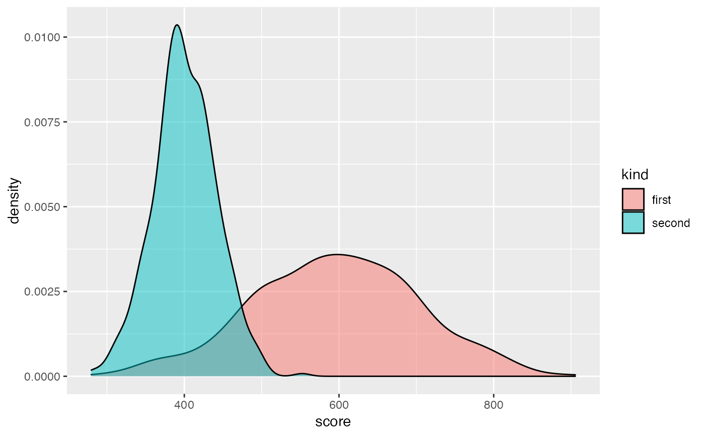
ggplot(custom_data, aes(score, fill = kind)) +
  geom_density(alpha = 0.5)


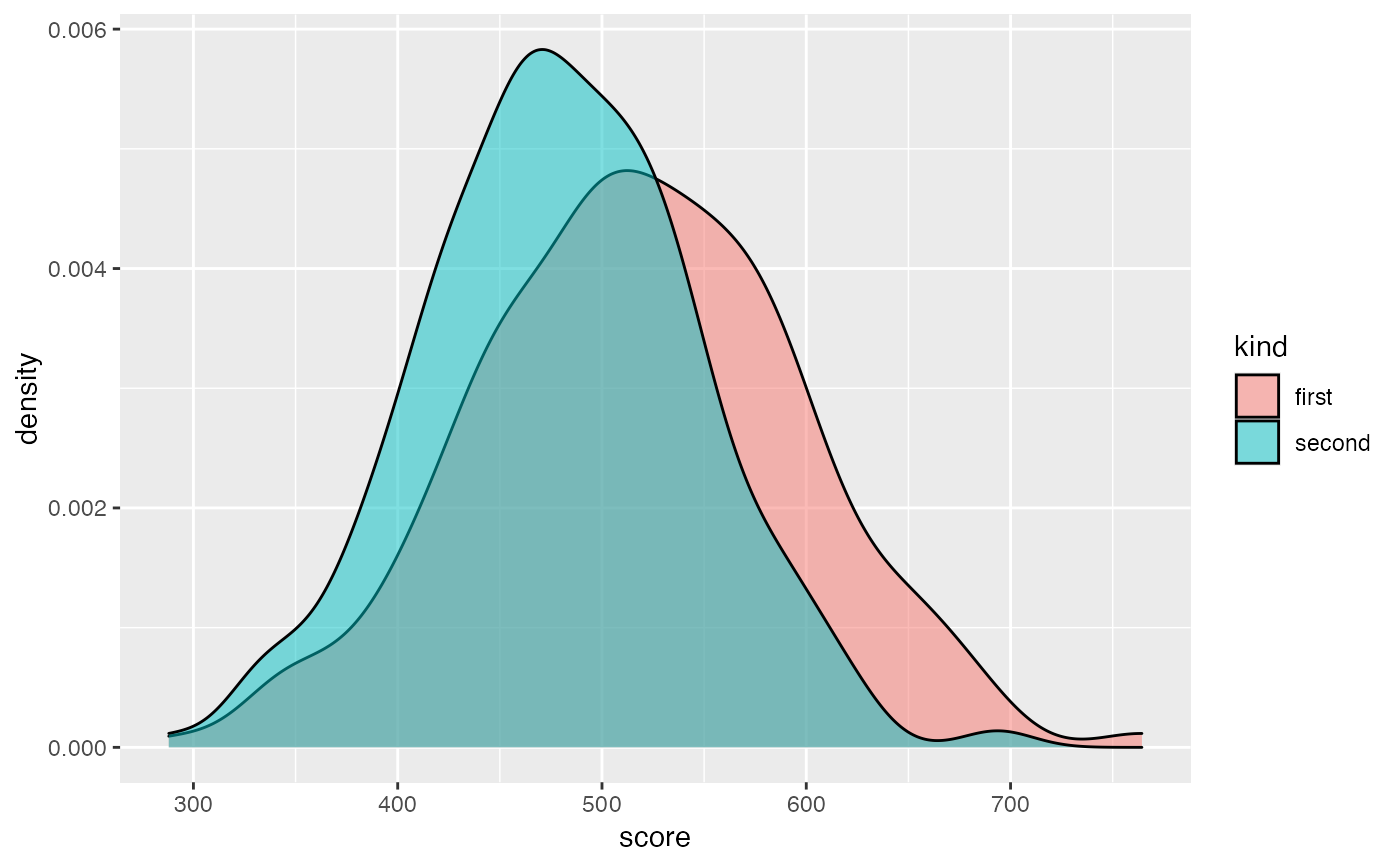
fixed_data <- disparate_impact_remover(
  data = custom_data,
  protected = custom_data$kind,
  features_to_transform = "score",
  lambda = 0.8
)

ggplot(fixed_data, aes(score, fill = kind)) +
  geom_density(alpha = 0.5)


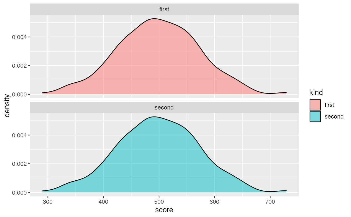
# lambda 1 gives identical distribution, lambda 0 (almost) original distributions

fixed_data_unchanged <- disparate_impact_remover(
  data = custom_data,
  protected = custom_data$kind,
  features_to_transform = "score",
  lambda = 0
)

ggplot(fixed_data_unchanged, aes(score, fill = kind)) +
  geom_density(alpha = 0.5)



fixed_data_fully_changed <- disparate_impact_remover(
  data = custom_data,
  protected = custom_data$kind,
  features_to_transform = "score",
  lambda = 1
)

ggplot(fixed_data_fully_changed, aes(score, fill = kind)) +
  geom_density(alpha = 0.5) +
  facet_wrap(kind ~ ., nrow = 2)