Local Conditional Expectation Explainer
This explainer works for individual observations. For each observation it calculates Local Conditional Expectation (LCE) profiles for selected variables.
individual_conditional_expectations(x, ...)

# S3 method for explainer
individual_conditional_expectations(x, new_observation,
  y = NULL, variables = NULL, variable_splits = NULL,
  grid_points = 101, ...)

# S3 method for default
individual_conditional_expectations(x, data,
  predict_function = predict, new_observation, y = NULL,
  variable_splits = NULL, variables = NULL, grid_points = 101,
  label = class(x)[1], ...)
Arguments
| x | a model to be explained, or an explainer created with function `DALEX::explain()`. |
|---|---|
| ... | other parameters |
| new_observation | a new observation with columns that corresponds to variables used in the model |
| y | true labels for `new_observation`. If specified then will be added to ceteris paribus plots. |
| variables | names of variables for which profiles shall be calculated. Will be passed to `calculate_variable_splits()`. If NULL then all variables from the validation data will be used. |
| variable_splits | named list of splits for variables, in most cases created with `calculate_variable_splits()`. If NULL then it will be calculated based on validation data avaliable in the `explainer`. |
| grid_points | number of points for profile. Will be passed to `calculate_variable_splits()`. |
| data | validation dataset, will be extracted from `x` if it's an explainer |
| predict_function | predict function, will be extracted from `x` if it's an explainer |
| label | name of the model. By default it's extracted from the 'class' attribute of the model |
Value
An object of the class 'individual_variable_profile_explainer'. A data frame with calculated LCE profiles.
Examples
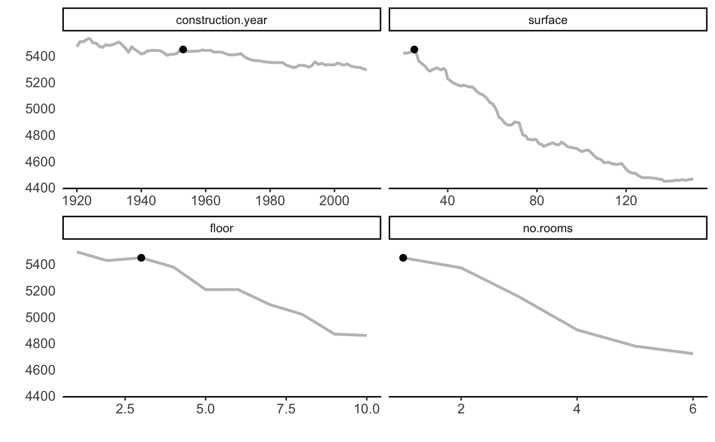
library("DALEX2")library("randomForest") set.seed(59) apartments_rf_model <- randomForest(m2.price ~ construction.year + surface + floor + no.rooms + district, data = apartments) explainer_rf <- explain(apartments_rf_model, data = apartments[,2:6], y = apartments$m2.price) new_apartment <- apartments[1, ] lce_rf <- individual_conditional_expectations(explainer_rf, new_apartment) lce_rf#> Top profiles : #> construction.year surface floor no.rooms district _yhat_ #> 1 1920 25 3 1 Srodmiescie 5467.437 #> 1.1 1921 25 3 1 Srodmiescie 5507.618 #> 1.2 1922 25 3 1 Srodmiescie 5505.886 #> 1.3 1923 25 3 1 Srodmiescie 5523.736 #> 1.4 1924 25 3 1 Srodmiescie 5530.727 #> 1.5 1925 25 3 1 Srodmiescie 5498.307 #> _vname_ _ids_ _label_ #> 1 construction.year 1 randomForest #> 1.1 construction.year 1 randomForest #> 1.2 construction.year 1 randomForest #> 1.3 construction.year 1 randomForest #> 1.4 construction.year 1 randomForest #> 1.5 construction.year 1 randomForest #> #> #> Top observations: #> construction.year surface floor no.rooms district _yhat_ _label_ #> 1 1953 25 3 1 Srodmiescie 5447.656 randomForest #> _ids_ #> 1 1lce_rf <- individual_conditional_expectations(explainer_rf, new_apartment, y = new_apartment$m2.price) lce_rf#> Top profiles : #> construction.year surface floor no.rooms district _yhat_ #> 1 1920 25 3 1 Srodmiescie 5467.437 #> 1.1 1921 25 3 1 Srodmiescie 5507.618 #> 1.2 1922 25 3 1 Srodmiescie 5505.886 #> 1.3 1923 25 3 1 Srodmiescie 5523.736 #> 1.4 1924 25 3 1 Srodmiescie 5530.727 #> 1.5 1925 25 3 1 Srodmiescie 5498.307 #> _vname_ _ids_ _label_ #> 1 construction.year 1 randomForest #> 1.1 construction.year 1 randomForest #> 1.2 construction.year 1 randomForest #> 1.3 construction.year 1 randomForest #> 1.4 construction.year 1 randomForest #> 1.5 construction.year 1 randomForest #> #> #> Top observations: #> construction.year surface floor no.rooms district _yhat_ _label_ #> 1 1953 25 3 1 Srodmiescie 5447.656 randomForest #> _ids_ _y_ #> 1 1 5897plot(lce_rf)