Plot importance of interactions or pairs
This function plots the importance ranking of interactions and pairs in the model.
# S3 method for interactions
plot(x, ...)
Arguments
| x | a result from the |
|---|---|
| ... | other parameters. |
Value
a ggplot object
Details
NOTE: Be careful use of this function with option="pairs" parameter,
because high gain of pair can be a result of high gain of child variable.
As strong interactions should be considered only these pairs of variables,
where variable on the bottom (child) has higher gain than variable on the top (parent).
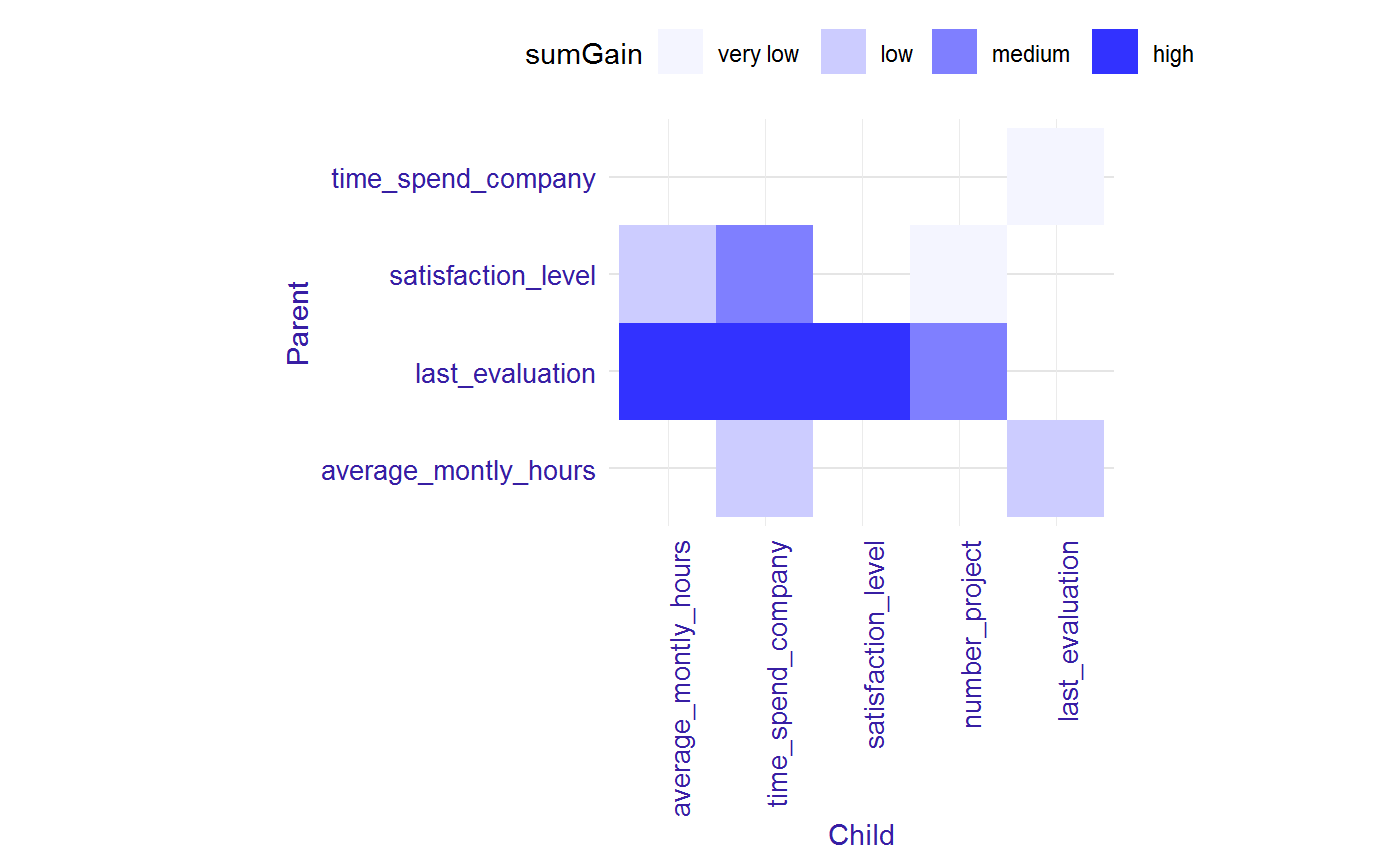
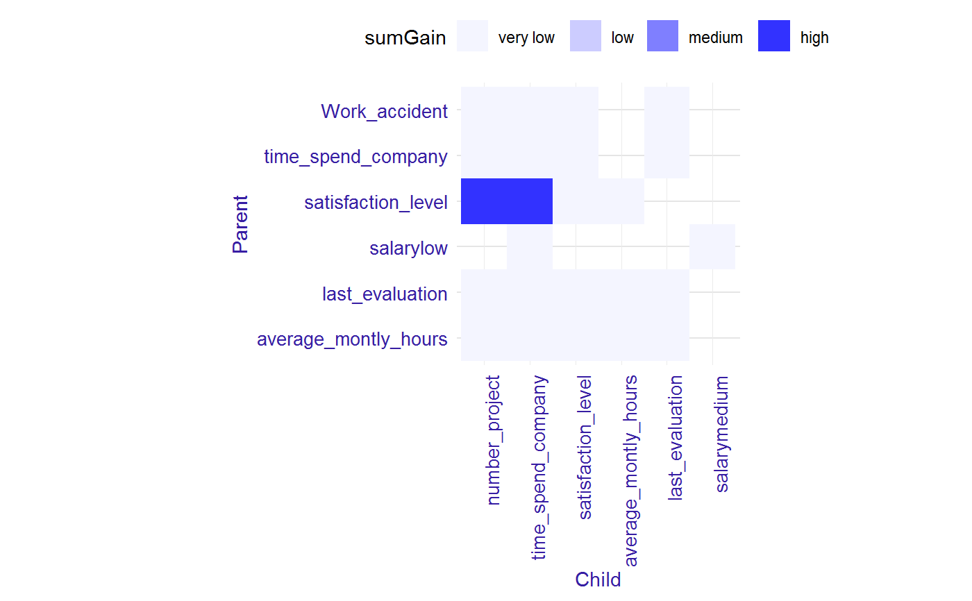
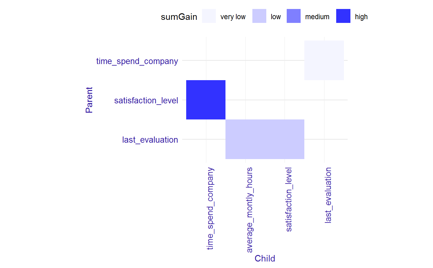
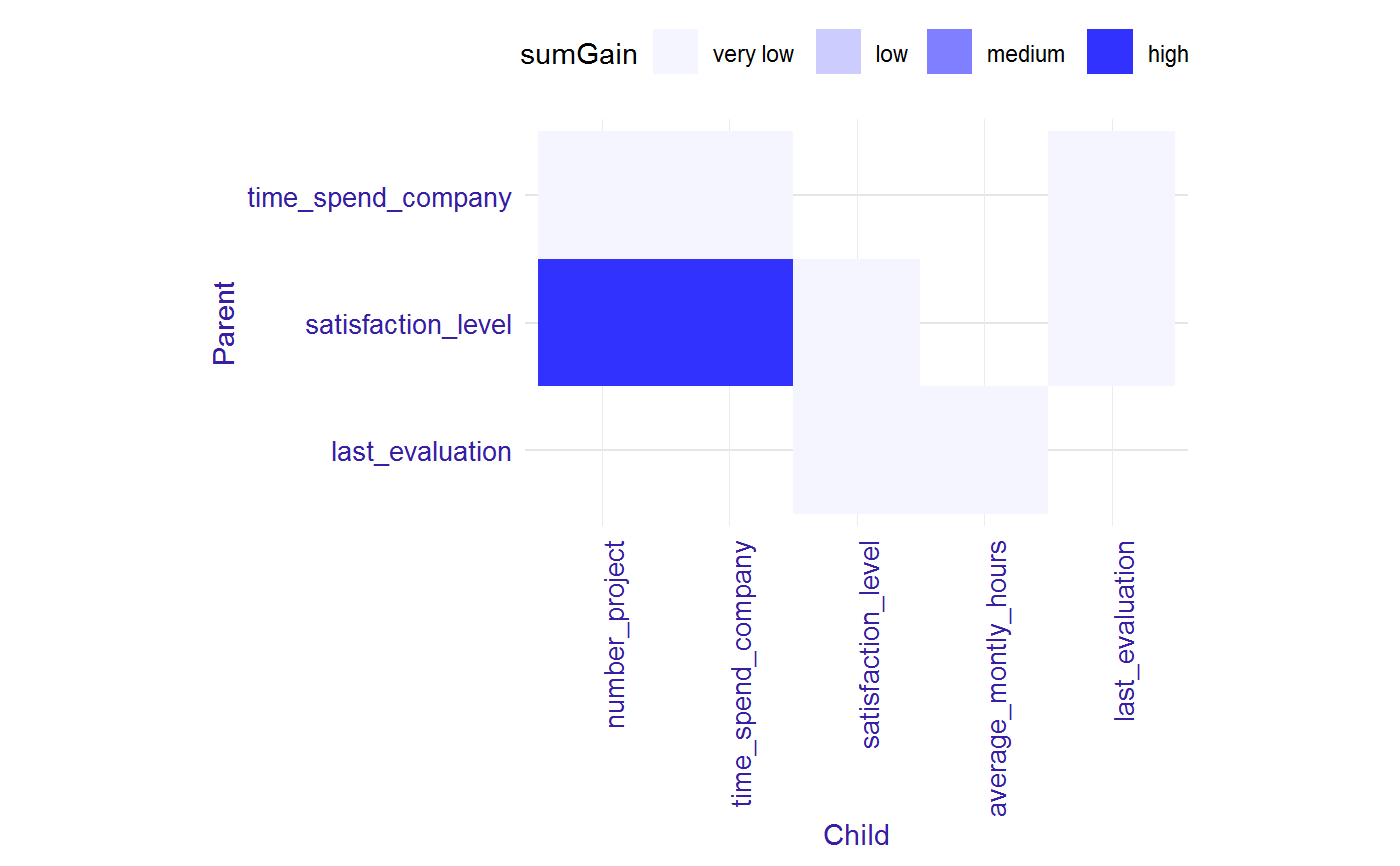
Examples
library("EIX") library("Matrix") sm <- sparse.model.matrix(left ~ . - 1, data = HR_data) library("xgboost") param <- list(objective = "binary:logistic", max_depth = 2) xgb_model <- xgboost(sm, params = param, label = HR_data[, left] == 1, nrounds = 25, verbose=0) inter <- interactions(xgb_model, sm, option = "interactions") inter#> Parent Child sumGain frequency #> 1: last_evaluation average_montly_hours 702.05170 1 #> 2: last_evaluation time_spend_company 564.30090 1 #> 3: last_evaluation satisfaction_level 502.90195 1 #> 4: last_evaluation number_project 390.18976 1 #> 5: satisfaction_level time_spend_company 332.18097 1 #> 6: average_montly_hours time_spend_company 262.55286 1 #> 7: average_montly_hours last_evaluation 249.13687 1 #> 8: satisfaction_level average_montly_hours 168.38992 1 #> 9: satisfaction_level number_project 87.09535 1 #> 10: time_spend_company last_evaluation 86.27449 1plot(inter)#> Parent Child sumGain frequency #> 1: satisfaction_level number_project 3573.869457 6 #> 2: satisfaction_level time_spend_company 3193.349916 4 #> 3: satisfaction_level satisfaction_level 820.880741 4 #> 4: last_evaluation average_montly_hours 767.932007 2 #> 5: last_evaluation satisfaction_level 616.821671 2 #> 6: last_evaluation time_spend_company 581.206291 2 #> 7: time_spend_company time_spend_company 404.105011 2 #> 8: last_evaluation number_project 399.432373 3 #> 9: average_montly_hours time_spend_company 262.552856 1 #> 10: average_montly_hours last_evaluation 249.136871 1 #> 11: satisfaction_level average_montly_hours 168.389923 1 #> 12: average_montly_hours satisfaction_level 139.267471 1 #> 13: last_evaluation last_evaluation 125.887398 1 #> 14: Work_accident number_project 119.155579 1 #> 15: average_montly_hours average_montly_hours 102.814651 1 #> 16: time_spend_company last_evaluation 86.274490 1 #> 17: salarylow time_spend_company 80.271004 1 #> 18: Work_accident time_spend_company 54.700195 1 #> 19: salarylow salarymedium 45.284599 1 #> 20: time_spend_company satisfaction_level 16.250031 1 #> 21: time_spend_company number_project 15.200378 1 #> 22: average_montly_hours number_project 14.579918 2 #> 23: Work_accident satisfaction_level 12.788223 1 #> 24: Work_accident last_evaluation 6.214535 1 #> Parent Child sumGain frequencyplot(inter)library(lightgbm) train_data <- lgb.Dataset(sm, label = HR_data[, left] == 1) params <- list(objective = "binary", max_depth = 2) lgb_model <- lgb.train(params, train_data, 25) inter <- interactions(lgb_model, sm, option = "interactions") inter#> Parent Child sumGain frequency #> 1: satisfaction_level time_spend_company 2434.0047 3 #> 2: last_evaluation average_montly_hours 658.0106 1 #> 3: last_evaluation satisfaction_level 539.9527 1 #> 4: time_spend_company last_evaluation 341.3317 1plot(inter)#> Parent Child sumGain frequency #> 1: satisfaction_level number_project 9845.23985 21 #> 2: satisfaction_level time_spend_company 8170.39149 10 #> 3: satisfaction_level satisfaction_level 1465.36041 2 #> 4: last_evaluation average_montly_hours 658.01062 1 #> 5: time_spend_company last_evaluation 612.09506 2 #> 6: last_evaluation satisfaction_level 539.95270 1 #> 7: time_spend_company time_spend_company 489.65636 2 #> 8: satisfaction_level last_evaluation 251.51668 7 #> 9: time_spend_company number_project 55.00172 4plot(inter)